❀编程理解❀从0搭建网络MobileNetV2并进行训练和测试

读懂mobilenetv2首先要了解的概念：深度可分离卷积Depthwise Separable Convolutions(DSC)，残差块（residual block）等

论文地址：[1801.04381] MobileNetV2: Inverted Residuals and Linear Bottlenecks (arxiv.org)

项目地址：pytorch框架

Randl/MobileNetV2-pytorch: Impementation of MobileNetV2 in pytorch (github.com)

1.MobileNetV2的主要思想

提出purpose:

提高移动模型的效率Improves the performance of mobile models

提出反残差块proposed model:Inverted Residual Block

2. 论文中的网络结构

2.1反残差结构Inverted Residual Block

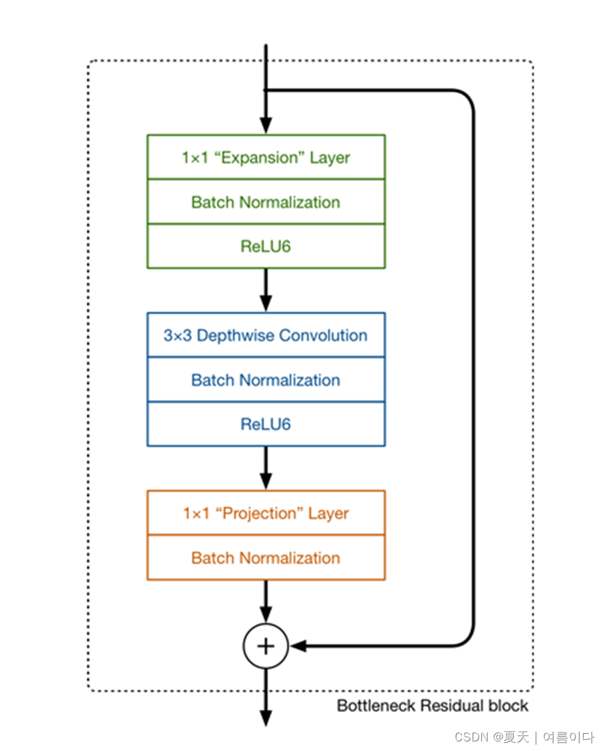
 This module takes as an input a low dim compressed representation which is first expanded to high dim and filtered with a light depthwise convolution.

该模块将低维度的压缩表示作为输入，首先将其扩展为高维度，并通过深度卷积进行过滤。

（在代码中是基本层+BN+ReLU6）

expansion factor指扩展因子（膨胀系数）

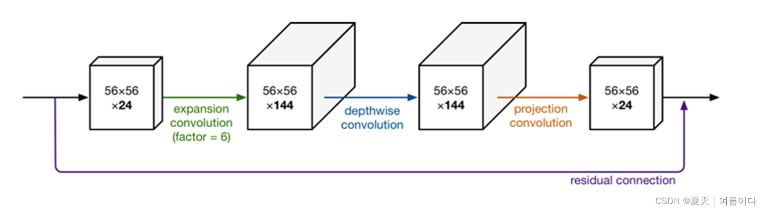
 先増维，后降维的情况和resnet block 先降维后増维的情况相反，所以叫inverted residual block,

2.2MobileNetV2网络框架

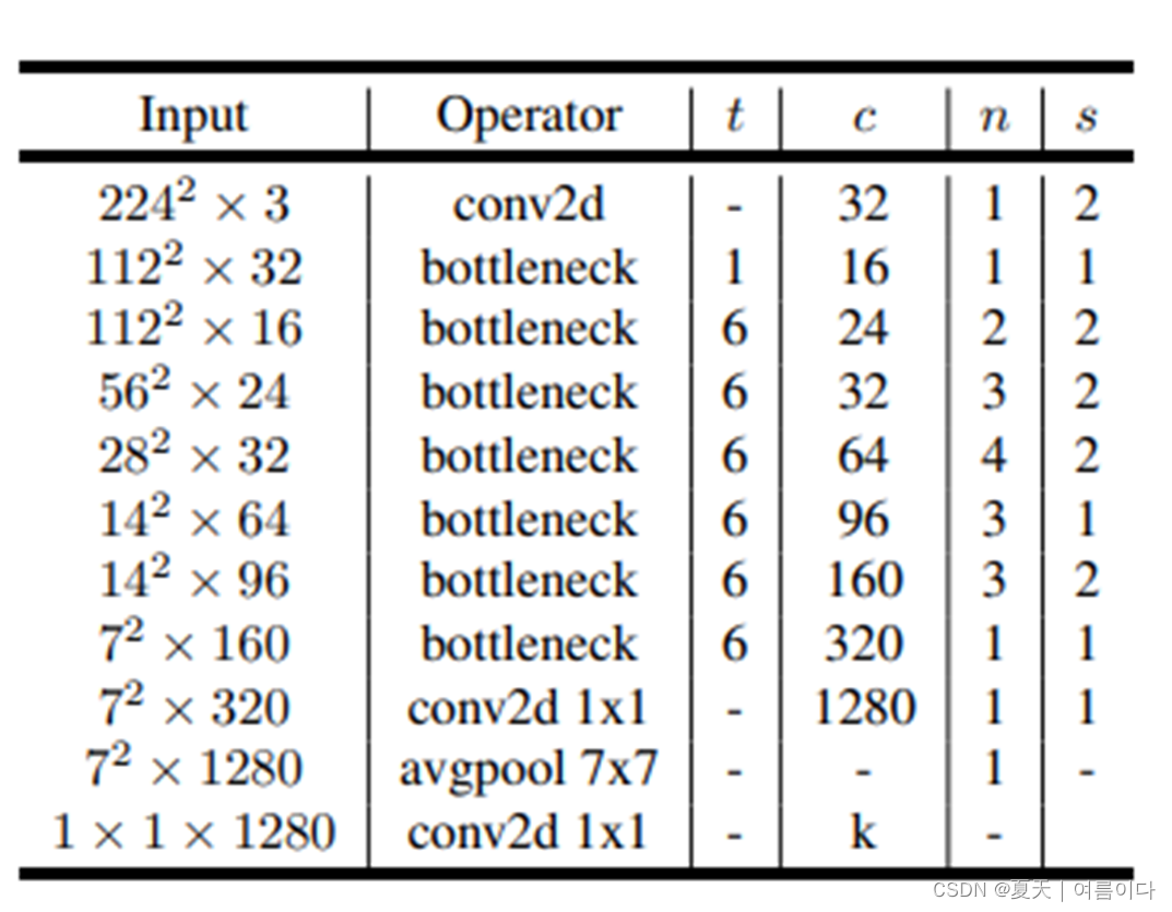
以反残差块为基础，构建MobileNetV2.

- t : 扩展因子（膨胀系数）expansion factor

- c : 输出通道数 number c of output channels

- n : 重复次数 number of repetitions

- s : 步长  stride

每个人的理解方式不同，按照我可以理解的方式搭建网络（个人觉得此代码更有助于理解论文）：

#step1 导入所需要的包
import torch
import torch.nn as nn
import torchvision.datasets as dsets
import torchvision.transforms as transforms
import torch.optim as optim
from torch.utils.data import DataLoader

#step2 定义device
device="cuda" if torch.cuda.is_available() else "cpu"

#step3 参数设置（学习率，训练轮数，批大小）
learning_rate=0.1
training_epochs=10
batch_size=16

#step4 Dataset & DataLoader设置数据集和数据加载器

trans=transforms.Compose([
    transforms.Resize((224,224)),
    transforms.ToTensor()
])
#DataSet设置数据集
cifar10_train=dsets.CIFAR10(root="cifar10_data",train=True,transform=trans,download=True)
cifar10_test=dsets.CIFAR10(root="cifar10_data",train=False,transform=trans,download=True)

#dataloader设置数据加载器
train_loader=DataLoader(dataset=cifar10_train,batch_size=batch_size,shuffle=True,drop_last=True)
test_loader=DataLoader(dataset=cifar10_test,batch_size=batch_size,shuffle=False,drop_last=False)


#step5 model定义层
def make_layers(cfg):
    in_channel=32
    layers=[]

    for v in cfg:
        t,out_channel,n,stride=v
        #编写深度可分离卷积DSC layer
        for i in range(n):
            if i !=0:
                stride=1
            conv_pointwise1=nn.Conv2d(in_channel,
                                      in_channel*t,
                                      kernel_size=1,
                                      stride=1,
                                      padding=0)
            conv_depthwise = nn.Conv2d(in_channel * t,
                                        in_channel * t,
                                        kernel_size=3,
                                        groups=in_channel*t,
                                        stride=stride,
                                        padding=1)
            conv_pointwise2 = nn.Conv2d(in_channel*t,
                                        out_channel ,
                                        kernel_size=1,
                                        stride=1,
                                        padding=0)
            #增加层之后的批量标准化和激活
            layers.append([conv_pointwise1,nn.BatchNorm2d(in_channel * t),nn.ReLU6(),
                           conv_depthwise, nn.BatchNorm2d(in_channel * t), nn.ReLU6(),
                           conv_pointwise2,nn.BatchNorm2d(out_channel)])
            in_channel=out_channel
    return layers

#定义网络
class Mobilenet(nn.Module):
    def __init__(self,features,stride_list,num_classes=10):
        super(Mobilenet, self).__init__()

        #conv2d
        self.layer1=nn.Sequential(
            nn.Conv2d(3,32,kernel_size=3,stride=2,padding=1),
            nn.BatchNorm2d(32),
        )
        #第一层卷积输入通道为3，输出通道为32，卷积核为3，步长为2，填充为1

        #bottleneck
        self.bottle_necks=[]
        for layer in features:
            self.bottle_necks.append(nn.Sequential(*layer).cuda())
        #论文中共17个bottleneck

        #last conv2d
        self.layer2=nn.Sequential(
            nn.Conv2d(320,1280,kernel_size=1,stride=1,padding=0),
            nn.BatchNorm2d(1280),
            nn.AvgPool2d(7,7),
        )
        #论文中的最后一个卷积和一个平均池化

        #classfier
        self.fc=nn.Linear(1280,num_classes)

    def forward(self,x):
        #layer1
        out=self.layer1(x)

        #bottlr_neck
        for i in range(len(self.bottle_necks)):
            new=self.bottle_necks[i](out)
            if stride_list[i]==1:#skip connection
                if out.shape[1]!=new.shape[1]:
                    out=Downsample(out.shape[1],new.shape[1]).cuda()(out)
                new+=out
            out=new

        # layer2
        #print("size",out.size())
        out = self.layer2(out)
        #fc
        out=out.view(out.size(0),-1)
        out=self.fc(out)

        return out

#当stride=2时，执行下采样
class Downsample(nn.Module):
    def __init__(self,in_channel,out_channel):
        super(Downsample, self).__init__()
        self.layer=nn.Sequential(
            nn.Conv2d(in_channel,out_channel,kernel_size=1),
            nn.BatchNorm2d(out_channel),
        )
    def forward(self,x):
        out=self.layer(x)
        return out
#   expansion factor扩展因子t，输出通道数c，重复次数n，步长s
cfg={'mobilenetv2':[(1,16,1,1),
                    (6,24,2,2),
                    (6,32,3,2),
                    (6,64,4,2),
                    (6,96,3,1),
                    (6,160,3,2),
                    (6,320,1,1)]}

bottleneck=make_layers(cfg["mobilenetv2"])

stride_list=[1,
             2,1,
             2,1,1,
             2,1,1,1,
             1,1,1,
             2,1,1,
             1]
model=Mobilenet(bottleneck,stride_list,num_classes=10).to(device)
model.cuda()
target=torch.Tensor(2,3,224,224).to(device)
#不能删掉batch_size

after_target=model(target)
print(after_target.shape)
print(after_target)

#step6 optim&loss优化器和函数
criterion=nn.CrossEntropyLoss().to(device)
optimizer=optim.Adam(model.parameters(),lr=learning_rate)


#step7 train训练
model.train()
iteration=len(train_loader)

for epoch in range(training_epochs):
    loss=0.0
    acc_correct=0.0

    for idx,sample in enumerate(train_loader):
        optimizer.zero_grad()
        X,Y=sample
        X=X.to(device)
        Y=Y.to(device)

        #foeward,backward,optim
        hypothesis=model(X)
        cost=criterion(hypothesis,Y)
        cost.backward()
        optimizer.step()

        #calculate
        loss+=cost.item()
        correct=(torch.argmax(hypothesis,dim=1)==Y).float()
        acc_correct+=correct.sum()
    acc_correct/=(batch_size*iteration)
    loss/=iteration
    print("[Epoch:{:04d}],loss:{:.2f},acc:{:.2f}%".format(epoch,loss,acc_correct*100))

#step8 test测试
with torch.no_grad():
    model.eval()
    accuracy=0
    loss=0
    for idx,sample in enumerate(test_loader):
        X,Y=sample
        X=X.to(device)
        Y=Y.to(device)


        hypothesis=model(X)
        cost=criterion(hypothesis,Y)

        #calculate
        loss+=cost.item()
        accuracy=(torch.argmax(hypothesis,dim=1)==Y).sum().float()

    acc_correct/=len(test_loader)
    accuracy/=(batch_size*len(test_loader))
    print("[test]loss:{:.4f},acc:{:.4f}%".format(loss/1000,acc_correct*1000))