


- 🍨 本文为🔗365天深度学习训练营 中的学习记录博客
- 🍖 原作者:K同学啊 | 接辅导、项目定制
- 🚀 文章来源:K同学的学习圈子
我的环境:
-
语言环境:python 3.8
-
编译器:jupyter notebook
-
深度学习环境:Pytorch
torch == 2.1.0+cpu
torchvision == 0.16.0+cpu
-
要求:
- 利用YOLOv5算法中的C3模块搭建网络,实现天气识别
一、准备工作
1. 导入库函数
import torch
import torch.nn as nn
import torchvision.transforms as transforms
import torchvision
from torchvision import transforms, datasets
import os,PIL,pathlib,warnings

warnings.filterwarnings("ignore")             #忽略警告信息

device = torch.device("cuda" if torch.cuda.is_available() else "cpu")
device
device(type='cpu')
2.加载数据
● 第一步:使用pathlib.Path()函数将字符串类型的文件夹路径转换为pathlib.Path对象。
● 第二步:使用glob()方法获取data_dir路径下的所有文件路径,并以列表形式存储在data_paths中。
● 第三步:通过split()函数对data_paths中的每个文件路径执行分割操作,获得各个文件所属的类别名称,并存储在classNames中
● 第四步:打印classNames列表,显示每个文件所属的类别名称。
import os,PIL,random,pathlib
data_dir = "D:\BaiduNetdiskDownload\datasets\weather_photos"
data_dir = pathlib.Path(data_dir)
data_paths = list(data_dir.glob('*/'))
classNames = [str(path).split("\\")[4] for path in data_paths]
classNames
['cloudy', 'rain', 'shine', 'sunrise']
3. 数据加载(设置batchsize和取样等功能)
# 关于transforms.Compose的更多介绍可以参考:https://blog.csdn.net/qq_38251616/article/details/124878863
train_transforms = transforms.Compose([
    transforms.Resize([224, 224]),  # 将输入图片resize成统一尺寸
    # transforms.RandomHorizontalFlip(), # 随机水平翻转
    transforms.ToTensor(),          # 将PIL Image或numpy.ndarray转换为tensor,并归一化到[0,1]之间
    transforms.Normalize(           # 标准化处理-->转换为标准正太分布(高斯分布),使模型更容易收敛
        mean=[0.485, 0.456, 0.406],
        std=[0.229, 0.224, 0.225])  # 其中 mean=[0.485,0.456,0.406]与std=[0.229,0.224,0.225] 从数据集中随机抽样计算得到的。
])

test_transform = transforms.Compose([
    transforms.Resize([224, 224]),  # 将输入图片resize成统一尺寸
    transforms.ToTensor(),          # 将PIL Image或numpy.ndarray转换为tensor,并归一化到[0,1]之间
    transforms.Normalize(           # 标准化处理-->转换为标准正太分布(高斯分布),使模型更容易收敛
        mean=[0.485, 0.456, 0.406],
        std=[0.229, 0.224, 0.225])  # 其中 mean=[0.485,0.456,0.406]与std=[0.229,0.224,0.225] 从数据集中随机抽样计算得到的。
])

total_data = datasets.ImageFolder("D:/BaiduNetdiskDownload/datasets/weather_photos",transform=train_transforms)
total_data
Dataset ImageFolder
    Number of datapoints: 1125
    Root location: D:/BaiduNetdiskDownload/datasets/weather_photos
    StandardTransform
Transform: Compose(
               Resize(size=[224, 224], interpolation=bilinear, max_size=None, antialias=warn)
               ToTensor()
               Normalize(mean=[0.485, 0.456, 0.406], std=[0.229, 0.224, 0.225])
           )
total_data.class_to_idx
{'cloudy': 0, 'rain': 1, 'shine': 2, 'sunrise': 3}
train_size = int(0.8 * len(total_data))
test_size  = len(total_data) - train_size
train_dataset, test_dataset = torch.utils.data.random_split(total_data, [train_size, test_size])
train_dataset, test_dataset
(<torch.utils.data.dataset.Subset at 0x199694d0d60>,
 <torch.utils.data.dataset.Subset at 0x1995fed6c40>)
batch_size = 4

train_dl = torch.utils.data.DataLoader(train_dataset,
                                       batch_size=batch_size,
                                       shuffle=True,
                                       num_workers=1)

test_dl  = torch.utils.data.DataLoader(test_dataset,
                                       batch_size=batch_size,
                                       shuffle=True,
                                       num_workers=1)
for X, y in test_dl:
    print("Shape of X [N, C, H, W]: ", X.shape)
    print("Shape of y: ", y.shape, y.dtype)
    break
Shape of X [N, C, H, W]:  torch.Size([4, 3, 224, 224])
Shape of y:  torch.Size([4]) torch.int64
二、搭建包含C3模块的模型
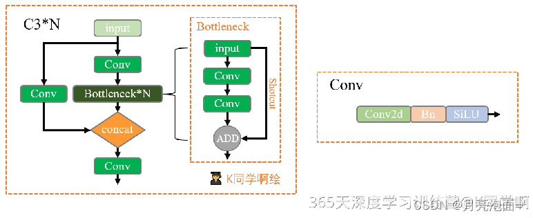
YOLOv5-C3模块是YOLOv5网络中的一个重要组成部分,其主要作用是增加网络的深度和感受野,提高特征提取的能力。
具体来说,YOLOv5-C3模块由三个Conv模块(Conv1、Conv2、Conv3)和多个Bottleneck模块组成的,因此,其结构可以大致分为四部分:
- Conv1:作为第一个Conv模块,它对输入的特征图进行一次卷积操作。这个卷积操作可以使用任意的卷积核,但根据设计,采用1*1的卷积核可以起到降维或升维的作用,对于提取特征有重要意义。
- Bottleneck:这是第二个模块,它包含两个部分。第一个部分是一个(1,1)的卷积,将输入特征图的通道数减半;第二部分是一个(3,3)的卷积,将通道数翻倍,最终输入和输出的通道数是不变的。shortcut参数控制是否进行残差链接。这种设计有利于增加网络的感受野,同时减少计算量。感受野的增加可以让网络更加关注物体的全局信息,从而提高特征提取的效果。
- Conv2和Conv3:这两个Conv模块的作用与Conv1类似,都是对特征图进行卷积操作。其中,Conv2的步幅为1,而Conv3的步幅为2。这样的设计也是为了增加网络的感受野。
在每个Conv模块之间,还加入了BN层和SiLU激活函数,以提高模型的稳定性和泛化性能。
总结起来,YOLOv5-C3模块通过多尺度特征融合技术和跨通道信息传递机制来提高特征图的表达能力,进而提升YOLOv5模型的性能和准确性。
1. 模型建立
import torch.nn.functional as F

def autopad(k, p=None):  # kernel, padding
    # Pad to 'same'
    if p is None:
        p = k // 2 if isinstance(k, int) else [x // 2 for x in k]  # auto-pad
    return p

class Conv(nn.Module):
    # Standard convolution
    def __init__(self, c1, c2, k=1, s=1, p=None, g=1, act=True):  # ch_in, ch_out, kernel, stride, padding, groups
        super().__init__()
        self.conv = nn.Conv2d(c1, c2, k, s, autopad(k, p), groups=g, bias=False)
        self.bn = nn.BatchNorm2d(c2)
        self.act = nn.SiLU() if act is True else (act if isinstance(act, nn.Module) else nn.Identity())

    def forward(self, x):
        return self.act(self.bn(self.conv(x)))

class Bottleneck(nn.Module):
    # Standard bottleneck
    def __init__(self, c1, c2, shortcut=True, g=1, e=0.5):  # ch_in, ch_out, shortcut, groups, expansion
        super().__init__()
        c_ = int(c2 * e)  # hidden channels
        self.cv1 = Conv(c1, c_, 1, 1)
        self.cv2 = Conv(c_, c2, 3, 1, g=g)
        self.add = shortcut and c1 == c2

    def forward(self, x):
        return x + self.cv2(self.cv1(x)) if self.add else self.cv2(self.cv1(x))

class C3(nn.Module):
    # CSP Bottleneck with 3 convolutions
    def __init__(self, c1, c2, n=1, shortcut=True, g=1, e=0.5):  # ch_in, ch_out, number, shortcut, groups, expansion
        super().__init__()
        c_ = int(c2 * e)  # hidden channels
        self.cv1 = Conv(c1, c_, 1, 1)
        self.cv2 = Conv(c1, c_, 1, 1)
        self.cv3 = Conv(2 * c_, c2, 1)  # act=FReLU(c2)
        self.m = nn.Sequential(*(Bottleneck(c_, c_, shortcut, g, e=1.0) for _ in range(n)))

    def forward(self, x):
        return self.cv3(torch.cat((self.m(self.cv1(x)), self.cv2(x)), dim=1))

class model_K(nn.Module):
    def __init__(self):
        super(model_K, self).__init__()

        # 卷积模块
        self.Conv = Conv(3, 32, 3, 2)

        # C3模块1
        self.C3_1 = C3(32, 64, 3, 2)

        # 全连接网络层,用于分类
        self.classifier = nn.Sequential(
            nn.Linear(in_features=802816, out_features=100),
            nn.ReLU(),
            nn.Linear(in_features=100, out_features=4)
        )

    def forward(self, x):
        x = self.Conv(x)
        x = self.C3_1(x)
        x = torch.flatten(x, start_dim=1)
        x = self.classifier(x)

        return x

device = "cuda" if torch.cuda.is_available() else "cpu"
print("Using {} device".format(device))

model = model_K().to(device)
model
Using cpu device


model_K(
  (Conv): Conv(
    (conv): Conv2d(3, 32, kernel_size=(3, 3), stride=(2, 2), padding=(1, 1), bias=False)
    (bn): BatchNorm2d(32, eps=1e-05, momentum=0.1, affine=True, track_running_stats=True)
    (act): SiLU()
  )
  (C3_1): C3(
    (cv1): Conv(
      (conv): Conv2d(32, 32, kernel_size=(1, 1), stride=(1, 1), bias=False)
      (bn): BatchNorm2d(32, eps=1e-05, momentum=0.1, affine=True, track_running_stats=True)
      (act): SiLU()
    )
    (cv2): Conv(
      (conv): Conv2d(32, 32, kernel_size=(1, 1), stride=(1, 1), bias=False)
      (bn): BatchNorm2d(32, eps=1e-05, momentum=0.1, affine=True, track_running_stats=True)
      (act): SiLU()
    )
    (cv3): Conv(
      (conv): Conv2d(64, 64, kernel_size=(1, 1), stride=(1, 1), bias=False)
      (bn): BatchNorm2d(64, eps=1e-05, momentum=0.1, affine=True, track_running_stats=True)
      (act): SiLU()
    )
    (m): Sequential(
      (0): Bottleneck(
        (cv1): Conv(
          (conv): Conv2d(32, 32, kernel_size=(1, 1), stride=(1, 1), bias=False)
          (bn): BatchNorm2d(32, eps=1e-05, momentum=0.1, affine=True, track_running_stats=True)
          (act): SiLU()
        )
        (cv2): Conv(
          (conv): Conv2d(32, 32, kernel_size=(3, 3), stride=(1, 1), padding=(1, 1), bias=False)
          (bn): BatchNorm2d(32, eps=1e-05, momentum=0.1, affine=True, track_running_stats=True)
          (act): SiLU()
        )
      )
      (1): Bottleneck(
        (cv1): Conv(
          (conv): Conv2d(32, 32, kernel_size=(1, 1), stride=(1, 1), bias=False)
          (bn): BatchNorm2d(32, eps=1e-05, momentum=0.1, affine=True, track_running_stats=True)
          (act): SiLU()
        )
        (cv2): Conv(
          (conv): Conv2d(32, 32, kernel_size=(3, 3), stride=(1, 1), padding=(1, 1), bias=False)
          (bn): BatchNorm2d(32, eps=1e-05, momentum=0.1, affine=True, track_running_stats=True)
          (act): SiLU()
        )
      )
      (2): Bottleneck(
        (cv1): Conv(
          (conv): Conv2d(32, 32, kernel_size=(1, 1), stride=(1, 1), bias=False)
          (bn): BatchNorm2d(32, eps=1e-05, momentum=0.1, affine=True, track_running_stats=True)
          (act): SiLU()
        )
        (cv2): Conv(
          (conv): Conv2d(32, 32, kernel_size=(3, 3), stride=(1, 1), padding=(1, 1), bias=False)
          (bn): BatchNorm2d(32, eps=1e-05, momentum=0.1, affine=True, track_running_stats=True)
          (act): SiLU()
        )
      )
    )
  )
  (classifier): Sequential(
    (0): Linear(in_features=802816, out_features=100, bias=True)
    (1): ReLU()
    (2): Linear(in_features=100, out_features=4, bias=True)
  )
)
# 统计模型参数量以及其他指标
import torchsummary as summary
summary.summary(model, (3, 224, 224))
----------------------------------------------------------------
        Layer (type)               Output Shape         Param #
================================================================
            Conv2d-1         [-1, 32, 112, 112]             864
       BatchNorm2d-2         [-1, 32, 112, 112]              64
              SiLU-3         [-1, 32, 112, 112]               0
              Conv-4         [-1, 32, 112, 112]               0
            Conv2d-5         [-1, 32, 112, 112]           1,024
       BatchNorm2d-6         [-1, 32, 112, 112]              64
              SiLU-7         [-1, 32, 112, 112]               0
              Conv-8         [-1, 32, 112, 112]               0
            Conv2d-9         [-1, 32, 112, 112]           1,024
      BatchNorm2d-10         [-1, 32, 112, 112]              64
             SiLU-11         [-1, 32, 112, 112]               0
             Conv-12         [-1, 32, 112, 112]               0
           Conv2d-13         [-1, 32, 112, 112]           9,216
      BatchNorm2d-14         [-1, 32, 112, 112]              64
             SiLU-15         [-1, 32, 112, 112]               0
             Conv-16         [-1, 32, 112, 112]               0
       Bottleneck-17         [-1, 32, 112, 112]               0
           Conv2d-18         [-1, 32, 112, 112]           1,024
      BatchNorm2d-19         [-1, 32, 112, 112]              64
             SiLU-20         [-1, 32, 112, 112]               0
             Conv-21         [-1, 32, 112, 112]               0
           Conv2d-22         [-1, 32, 112, 112]           9,216
      BatchNorm2d-23         [-1, 32, 112, 112]              64
             SiLU-24         [-1, 32, 112, 112]               0
             Conv-25         [-1, 32, 112, 112]               0
       Bottleneck-26         [-1, 32, 112, 112]               0
           Conv2d-27         [-1, 32, 112, 112]           1,024
      BatchNorm2d-28         [-1, 32, 112, 112]              64
             SiLU-29         [-1, 32, 112, 112]               0
             Conv-30         [-1, 32, 112, 112]               0
           Conv2d-31         [-1, 32, 112, 112]           9,216
      BatchNorm2d-32         [-1, 32, 112, 112]              64
             SiLU-33         [-1, 32, 112, 112]               0
             Conv-34         [-1, 32, 112, 112]               0
       Bottleneck-35         [-1, 32, 112, 112]               0
           Conv2d-36         [-1, 32, 112, 112]           1,024
      BatchNorm2d-37         [-1, 32, 112, 112]              64
             SiLU-38         [-1, 32, 112, 112]               0
             Conv-39         [-1, 32, 112, 112]               0
           Conv2d-40         [-1, 64, 112, 112]           4,096
      BatchNorm2d-41         [-1, 64, 112, 112]             128
             SiLU-42         [-1, 64, 112, 112]               0
             Conv-43         [-1, 64, 112, 112]               0
               C3-44         [-1, 64, 112, 112]               0
           Linear-45                  [-1, 100]      80,281,700
             ReLU-46                  [-1, 100]               0
           Linear-47                    [-1, 4]             404
================================================================
Total params: 80,320,536
Trainable params: 80,320,536
Non-trainable params: 0
----------------------------------------------------------------
Input size (MB): 0.57
Forward/backward pass size (MB): 150.06
Params size (MB): 306.40
Estimated Total Size (MB): 457.04
----------------------------------------------------------------
2. 训练函数
2.1 训练函数
- optimizer.zero_grad(),梯度清零。
- loss.backward(),反向传播计算每个w的梯度值。
- optimizer.step(),梯度下降法更新参数值。
# 训练循环
def train(dataloader, model, loss_fn, optimizer):
    size = len(dataloader.dataset)  # 训练集的大小,一共60000张图片
    num_batches = len(dataloader)   # 批次数目,1875(60000/32)

    train_loss, train_acc = 0, 0  # 初始化训练损失和正确率

    for X, y in dataloader:  # 获取图片及其标签
        X, y = X.to(device), y.to(device)

        # 计算预测误差
        pred = model(X)          # 网络输出
        loss = loss_fn(pred, y)  # 计算网络输出和真实值之间的差距,targets为真实值,计算二者差值即为损失

        # 反向传播
        optimizer.zero_grad()  # grad属性归零
        loss.backward()        # 反向传播
        optimizer.step()       # 每一步自动更新

        # 记录acc与loss
        train_acc  += (pred.argmax(1) == y).type(torch.float).sum().item()
        train_loss += loss.item()

    train_acc  /= size
    train_loss /= num_batches

    return train_acc, train_loss
train_acc和loss的计算原理:
- pred.argmax(1)返回预测结果pred行最大值的索引,每行是表示一个样本的预测概率分布。==y表示判断预测是否正确。
- .type(torch.float)将判断结果转为浮点类型可以进行求和。
- .sum()对预测结果的正误进行求和。
- .item()将求和结果转为标量值便于输出。
2.2 测试函数
去掉了训练函数中梯度下降和权重更新的步骤。
def test (dataloader, model, loss_fn):
    size        = len(dataloader.dataset)  # 测试集的大小,一共10000张图片
    num_batches = len(dataloader)          # 批次数目,313(10000/32=312.5,向上取整)
    test_loss, test_acc = 0, 0

    # 当不进行训练时,停止梯度更新,节省计算内存消耗
    with torch.no_grad():
        for imgs, target in dataloader:
            imgs, target = imgs.to(device), target.to(device)

            # 计算loss
            target_pred = model(imgs)
            loss        = loss_fn(target_pred, target)

            test_loss += loss.item()
            test_acc  += (target_pred.argmax(1) == target).type(torch.float).sum().item()

    test_acc  /= size
    test_loss /= num_batches

    return test_acc, test_loss
2.4 模型训练
- model.train(),用于训练,启用BN层和dropout。
- model.eval(),用于测试,不启用BN层和dropout。
import copy

optimizer  = torch.optim.Adam(model.parameters(), lr= 1e-4)
loss_fn    = nn.CrossEntropyLoss() # 创建损失函数

epochs     = 20

train_loss = []
train_acc  = []
test_loss  = []
test_acc   = []

best_acc = 0    # 设置一个最佳准确率,作为最佳模型的判别指标

for epoch in range(epochs):

    model.train()
    epoch_train_acc, epoch_train_loss = train(train_dl, model, loss_fn, optimizer)

    model.eval()
    epoch_test_acc, epoch_test_loss = test(test_dl, model, loss_fn)

    # 保存最佳模型到 best_model
    if epoch_test_acc > best_acc:
        best_acc   = epoch_test_acc
        best_model = copy.deepcopy(model)

    train_acc.append(epoch_train_acc)
    train_loss.append(epoch_train_loss)
    test_acc.append(epoch_test_acc)
    test_loss.append(epoch_test_loss)

    # 获取当前的学习率
    lr = optimizer.state_dict()['param_groups'][0]['lr']

    template = ('Epoch:{:2d}, Train_acc:{:.1f}%, Train_loss:{:.3f}, Test_acc:{:.1f}%, Test_loss:{:.3f}, Lr:{:.2E}')
    print(template.format(epoch+1, epoch_train_acc*100, epoch_train_loss,
                          epoch_test_acc*100, epoch_test_loss, lr))

# 保存最佳模型到文件中
PATH = './best_model.pth'  # 保存的参数文件名
torch.save(model.state_dict(), PATH)

print('Done')
Epoch: 1, Train_acc:71.8%, Train_loss:1.286, Test_acc:81.8%, Test_loss:0.446, Lr:1.00E-04
Epoch: 2, Train_acc:88.8%, Train_loss:0.374, Test_acc:83.1%, Test_loss:0.464, Lr:1.00E-04
Epoch: 3, Train_acc:92.3%, Train_loss:0.241, Test_acc:79.6%, Test_loss:0.554, Lr:1.00E-04
Epoch: 4, Train_acc:94.1%, Train_loss:0.166, Test_acc:85.8%, Test_loss:0.420, Lr:1.00E-04
Epoch: 5, Train_acc:97.6%, Train_loss:0.094, Test_acc:87.6%, Test_loss:0.412, Lr:1.00E-04
Epoch: 6, Train_acc:98.8%, Train_loss:0.035, Test_acc:88.0%, Test_loss:0.355, Lr:1.00E-04
Epoch: 7, Train_acc:99.2%, Train_loss:0.022, Test_acc:86.2%, Test_loss:0.404, Lr:1.00E-04
Epoch: 8, Train_acc:99.3%, Train_loss:0.019, Test_acc:88.4%, Test_loss:0.364, Lr:1.00E-04
Epoch: 9, Train_acc:97.9%, Train_loss:0.078, Test_acc:84.9%, Test_loss:0.547, Lr:1.00E-04
Epoch:10, Train_acc:97.3%, Train_loss:0.104, Test_acc:85.3%, Test_loss:0.562, Lr:1.00E-04
Epoch:11, Train_acc:98.2%, Train_loss:0.053, Test_acc:85.8%, Test_loss:0.421, Lr:1.00E-04
Epoch:12, Train_acc:99.3%, Train_loss:0.039, Test_acc:88.0%, Test_loss:0.570, Lr:1.00E-04
Epoch:13, Train_acc:98.9%, Train_loss:0.048, Test_acc:88.4%, Test_loss:0.424, Lr:1.00E-04
Epoch:14, Train_acc:99.3%, Train_loss:0.026, Test_acc:88.0%, Test_loss:0.479, Lr:1.00E-04
Epoch:15, Train_acc:99.4%, Train_loss:0.014, Test_acc:85.3%, Test_loss:0.621, Lr:1.00E-04
Epoch:16, Train_acc:99.9%, Train_loss:0.004, Test_acc:88.9%, Test_loss:0.544, Lr:1.00E-04
Epoch:17, Train_acc:98.7%, Train_loss:0.037, Test_acc:84.4%, Test_loss:0.739, Lr:1.00E-04
Epoch:18, Train_acc:99.4%, Train_loss:0.016, Test_acc:85.3%, Test_loss:0.788, Lr:1.00E-04
Epoch:19, Train_acc:98.9%, Train_loss:0.058, Test_acc:81.3%, Test_loss:1.114, Lr:1.00E-04
Epoch:20, Train_acc:96.8%, Train_loss:0.158, Test_acc:85.3%, Test_loss:1.086, Lr:1.00E-04
Done
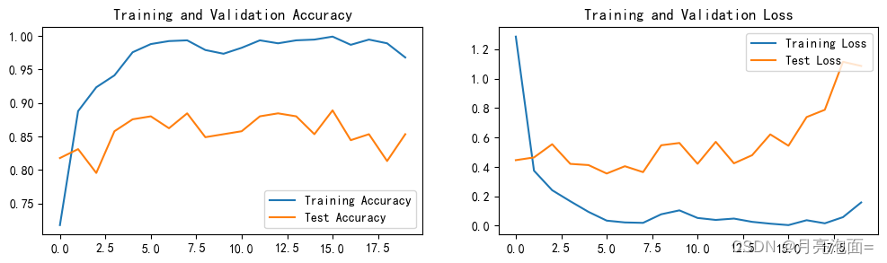
三、训练结果
1. loss and accuracy
import matplotlib.pyplot as plt
#隐藏警告
import warnings
warnings.filterwarnings("ignore")               #忽略警告信息
plt.rcParams['font.sans-serif']    = ['SimHei'] # 用来正常显示中文标签
plt.rcParams['axes.unicode_minus'] = False      # 用来正常显示负号
plt.rcParams['figure.dpi']         = 100        #分辨率

epochs_range = range(epochs)

plt.figure(figsize=(12, 3))
plt.subplot(1, 2, 1)

plt.plot(epochs_range, train_acc, label='Training Accuracy')
plt.plot(epochs_range, test_acc, label='Test Accuracy')
plt.legend(loc='lower right')
plt.title('Training and Validation Accuracy')

plt.subplot(1, 2, 2)
plt.plot(epochs_range, train_loss, label='Training Loss')
plt.plot(epochs_range, test_loss, label='Test Loss')
plt.legend(loc='upper right')
plt.title('Training and Validation Loss')
plt.show()
3. 模型评估
best_model.eval()
epoch_test_acc, epoch_test_loss = test(test_dl, best_model, loss_fn)
epoch_test_acc, epoch_test_loss
(0.8888888888888888, 0.5540382709102737)
best_acc
0.8888888888888888
四、总结
- 学习了YOLOv5的C3模块的搭建,详细知识见模型建立部分。


 860
860


 被折叠的 条评论
为什么被折叠?
被折叠的 条评论
为什么被折叠?
 到【灌水乐园】发言


