


根据点云生成贝塞尔曲面,官方文档见:
https://nurbs-python.readthedocs.io/en/5.x/visualization.html#surfaces
用Conda安装
NURBS-Python can also be installed/upgraded via conda package manager from the Anaconda Cloud repository.
Installing:
$ conda install -c orbingol geomdl
这里有源码:nurbs-python.readthedocs.io/en/5.x/visualization-3.py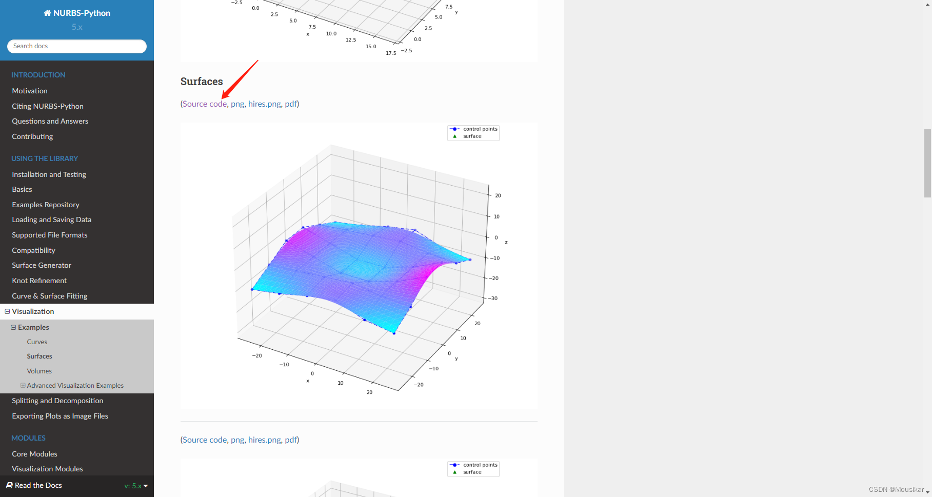
运行发现没有图像显示
就很蒙圈啊啊!
于是参考github的例子:geomdl-examples/fitting/approximation/global_surface.py at master · orbingol/geomdl-examples · GitHub
把可视化改一改,得到如下代码:
import geomdl
print(geomdl.__version__)
from geomdl import BSpline
from geomdl.visualization import VisMPL

# Control points
ctrlpts = [
    [[-25.0, -25.0, -10.0], [-25.0, -15.0, -5.0], [-25.0, -5.0, 0.0], [-25.0, 5.0, 0.0], [-25.0, 15.0, -5.0], [-25.0, 25.0, -10.0]],
    [[-15.0, -25.0, -8.0], [-15.0, -15.0, -4.0], [-15.0, -5.0, -4.0], [-15.0, 5.0, -4.0], [-15.0, 15.0, -4.0], [-15.0, 25.0, -8.0]],
    [[-5.0, -25.0, -5.0], [-5.0, -15.0, -3.0], [-5.0, -5.0, -8.0], [-5.0, 5.0, -8.0], [-5.0, 15.0, -3.0], [-5.0, 25.0, -5.0]],
    [[5.0, -25.0, -3.0], [5.0, -15.0, -2.0], [5.0, -5.0, -8.0], [5.0, 5.0, -8.0], [5.0, 15.0, -2.0], [5.0, 25.0, -3.0]],
    [[15.0, -25.0, -8.0], [15.0, -15.0, -4.0], [15.0, -5.0, -4.0], [15.0, 5.0, -4.0], [15.0, 15.0, -4.0], [15.0, 25.0, -8.0]],
    [[25.0, -25.0, -10.0], [25.0, -15.0, -5.0], [25.0, -5.0, 2.0], [25.0, 5.0, 2.0], [25.0, 15.0, -5.0], [25.0, 25.0, -10.0]]
]

# Create a BSpline surface
surf = BSpline.Surface()

# Set degrees
surf.degree_u = 3
surf.degree_v = 3

# Set control points
surf.ctrlpts2d = ctrlpts

# Set knot vectors
surf.knotvector_u = [0.0, 0.0, 0.0, 0.0, 1.0, 2.0, 3.0, 3.0, 3.0, 3.0]
surf.knotvector_v = [0.0, 0.0, 0.0, 0.0, 1.0, 2.0, 3.0, 3.0, 3.0, 3.0]

# Set evaluation delta
surf.delta = 0.025

# Evaluate surface points
surf.evaluate()

# Import and use Matplotlib's colormaps
from matplotlib import cm

# Plot the control points grid and the evaluated surface
surf.vis = VisMPL.VisSurface()
surf.render(colormap=cm.cool)


# # Visualize data and evaluated points together
import numpy as np
import matplotlib.pyplot as plt
evalpts = np.array(surf.evalpts)
pts=[]
for i in range(len(ctrlpts)):
    for j in range(len(ctrlpts[1])):
        pts.append(ctrlpts[i][j])

pts = np.array(pts)
print(pts[:, 0])
fig = plt.figure()
ax = plt.axes(projection='3d')
ax.scatter(evalpts[:, 0], evalpts[:, 1], evalpts[:, 2])
ax.scatter(pts[:, 0], pts[:, 1], pts[:, 2], color="red")
plt.show()
终于得到了图像: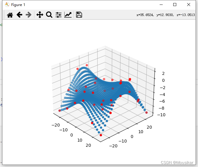


 845
845

 被折叠的 条评论
为什么被折叠?
被折叠的 条评论
为什么被折叠?
 到【灌水乐园】发言


