


目录
题目
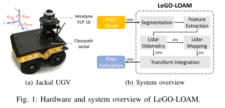
LeGO-LOAM: Lightweight and Ground-Optimized Lidar Odometry and Mapping on Variable Terrain
:在可变地形上的轻量级的利用地面点优化的Iidar 里程计和 建图模块
The code for LeGO-LOAM is available at https://github.com/RobustFieldAutonomyLab/LeGO-LOAM
The paper for LeGO-LOAM is available at : https://github.com/RobustFieldAutonomyLab/LeGO-LOAM/blob/master/Shan_Englot_IROS_2018_Preprint.pdf
Abstract
We propose a lightweight and ground-optimized lidar odometry and mapping method, LeGO-LOAM, for realtime six degree-of-freedom pose estimation with ground vehicles. LeGO-LOAM is lightweight, as it can achieve realtime pose estimation on a low-power embedded system. LeGOLOAM is ground-optimized, as it leverages the presence of a ground plane in its segmentation and optimization steps. We first apply point cloud segmentation to filter out noise, and feature extraction to obtain distinctive planar and edge features. A two-step Levenberg-Marquardt optimization method then uses the planar and edge features to solve different components of the six degree-of-freedom transformation across consecutive scans. We compare the performance of LeGO-LOAM with a state-of-the-art method, LOAM, using datasets gathered from variable-terrain environments with ground vehicles, and show that LeGO-LOAM achieves similar or better accuracy with reduced computational expense. We also integrate LeGO-LOAM into a SLAM framework to eliminate the pose estimation error caused by drift, which is tested using the KITTI dataset.
我们提出了一种轻型和基于地面优化的激光雷达里程计和建图的方法LeGO-LOAM,用于地面车辆的实时六自由度姿态估计。LeGO-LOAM是轻量的,可以在低功耗嵌入式系统上实现实时姿态估计。LeGOLOAM是基于地面优化的,它在分割和优化步骤中利用了地面。我们首先应用点云分割来滤除噪声,然后进行特征提取以获得不同的平面和边缘特征。然后,利用平面和边缘特征采用了两步Levenberg-Marquardt优化方法,来求解连续扫描中六自由度变换的不同分量。我们使用车辆在不同地形环境中收集的数据集,将LeGO-LOAM的性能与LOAM进行了比较,结果表明,LeGO-LOAM在降低计算开支的情况下达到了与LOAM类似或更好的精度。我们还将LeGO-LOAM集成到SLAM框架中,以消除漂移引起的姿态估计误差,并使用KITTI数据集进行了测试。
专为水平安装的Lidar设计的一个算法
I. Introduction
Among the capabilities of an intelligent robot, map building and state estimation are among the most fundamental prerequisites. Great efforts have been devoted to achieving real-time 6 degree-of-freedom simultaneous localization and mapping (SLAM) with vision-based and lidar-based methods. Although vision-based methods have advantages in loop-closure detection, their sensitivity to illumination and viewpoint change may make such capabilities unreliable if used as the sole navigation sensor. On the other hand, lidar based methods will function even at night, and the high resolution of many 3D lidars permits the capture of the fine details of an environment at long ranges, over a wide aperture. Therefore, this paper focuses on using 3D lidar to support real-time state estimation and mapping.
对于智能机器人而言,地图构建和状态估计是最基本的先决要求之一。人们一直致力于利用基于视觉和基于激光雷达的方法实现实时6自由度同步定位和建图(SLAM)。尽管基于视觉的方法在回环检测方面具有优势,但如果将其用作唯一的导航传感器,相机对于照明和视点变化的敏感性可能会使此类功能不可靠。另一方面,基于激光雷达的方法即使在夜间也能发挥作用,许多3D激光雷达的高分辨率允许在大孔径上远距离捕捉环境的细节。因此,本文主要研究利用三维激光雷达来实现SLAM。
The typical approach for finding the transformation between two lidar scans is iterative closest point (ICP) [1]. By finding correspondences at a point-wise level, ICP aligns two sets of points iteratively until stopping criteria are satisfied. When the scans include large quantities of points, ICP may suffer from prohibitive computational cost. Many variants of ICP have been proposed to improve its efficiency and accuracy [2]. [3] introduces a point-to-plane ICP variant that matches points to local planar patches. Generalized-ICP [4] proposes a method that matches local planar patches from both scans. In addition, several ICP variants have leveraged parallel computing for improved efficiency [5]–[8].
寻找两次激光雷达扫描之间位姿变换的典型方法是迭代最近邻(ICP)[1]。通过逐点查找对应关系,ICP迭代对齐两组点,直到满足停止条件为止。当扫描包含大量的点时,ICP可能会承受高昂的计算成本。为了提高ICP的效率和准确性,已经提出了许多ICP变体[2]。[3] 介绍一种点到平面ICP变体,该方法将点与局部平面面片相匹配。广义ICP[4]提出了一种匹配两次扫描的局部平面面片的方法。此外,几个ICP变种利用了并行计算来提高效率[5]–[8]。
Feature-based matching methods are attracting more attention, as they require less computational resources by extracting representative features from the environment. These features should be suitable for effective matching and invariant of point-of-view. Many detectors, such as Point Feature Histograms (PFH) [9] and Viewpoint Feature Histograms (VFH) [10], have been proposed for extracting such features from point clouds using simple and efficient techniques. A method for extracting general-purpose features from point clouds using a Kanade-Tomasi corner detector is introduced in [11]. A framework for extracting line and plane features from dense point clouds is discussed in [12].
基于特征的匹配方法越来越受到人们的关注,因为它们通过从环境中提取具有代表性的特征来减少计算资源。这些特征应适用于有效匹配和视点不变性。社区已经提出了许多检测器,例如点特征直方图(PFH)[9]和视点特征直方图(VFH)[10],用于使用简单有效的技术从点云中提取此类特征。[11]介绍了一种使用Kanade-Tomasi角点检测器从点云中提取通用特征的方法。[12]讨论了从密集点云中提取直线和平面特征的框架。
Many algorithms that use features for point cloud registration have also been proposed. [13] and [14] present a keypoint selection algorithm that performs point curvature calculations in a local cluster. The selected keypoints are then used to perform matching and place recognition. By projecting a point cloud onto a range image and analyzing the second derivative of the depth values, [15] selects features from points that have high curvature for matching and place recognition. Assuming the environment is composed of planes, a plane-based registration algorithm is proposed in [16]. An outdoor environment, e.g., a forest, may limit the application of such a method. A collar line segments (CLS) method, which is especially designed for Velodyne lidar, is presented in [17]. CLS randomly generates lines using points from two consecutive “rings” of a scan. Thus two line clouds are generated and used for registration. However, this method suffers from challenges arising from the random generation of lines. A segmentation-based registration algorithm is proposed in [18]. SegMatch first applies segmentation to a point cloud. Then a feature vector is calculated for each segment based on its eigenvalues and shape histograms. A random forest is used to match the segments from two scans. Though this method can be used for online pose estimation, it can only provide localization updates at about 1Hz.
社区还提出了许多使用特征进行点云配准的算法。[13] [14]提出了一种关键点选择算法,该算法在局部簇中执行点曲率计算。然后使用选定的关键点执行匹配和位置识别。通过将点云投影到距离图像上并分析深度值的二阶导数,[15]从具有高曲率的点中选择特征进行匹配和位置识别。假设环境由平面组成,在[16]中提出了一种基于平面的配准算法。室外环境,例如森林,可能会限制这种方法的应用。文献[17]中介绍了专门为Velodyne激光雷达设计的项圈线段(CLS)方法。CLS使用扫描的两个连续“环”中的点随机生成线。因此,将生成两个线云并用于注册。然而,这种方法受到随机生成线的挑战。文献[18]提出了一种基于分割的配准算法。SegMatch首先将分段应用于点云。然后根据特征值和形状直方图计算每个线段的特征向量。随机林用于匹配两次扫描的段。虽然这种方法可以用于在线姿态估计,但它只能提供1Hz左右的定位更新。
A low-drift and real-time lidar odometry and mapping (LOAM) method is proposed in [19] and [20]. LOAM performs point feature to edge/plane scan-matching to find correspondences between scans. Features are extracted by calculating the roughness of a point in its local region. The points with high roughness values are selected as edge features. Similarly, the points with low roughness values are designated planar features. Real-time performance is achieved by novelly dividing the estimation problem across two individual algorithms. One algorithm runs at high frequency and estimates sensor velocity at low accuracy. The other algorithm runs at low frequency but returns high-accuracy motion estimation. The two estimates are fused together to produce a single motion estimate at both high frequency and high accuracy. LOAM’s resulting accuracy is the best achieved by a lidar-only estimation method on the KITTI odometry benchmark site [21].
[19]和[20]中提出了一种低漂移实时激光雷达里程计和建图(LOAM)方法。LOAM执行点特征到边/平面的扫描匹配,以查找扫描之间的对应关系。通过计算局部点的曲率(roughness) 来提取特征。选择曲率(roughness)较高的点作为边缘特征。同样,曲率(roughness)较低的点被指定为平面特征。实时性能是通过将估计问题分为两个单独的算法来实现的。一种算法运行频率高,以较低的精度估计传感器的速度。另一种算法运行频率较低,但可以以高精度获得运动估计。将这两个估计值融合在一起,以产生高频和高精度的单个运动估计值。在KITTI里程计基准点上,通过仅使用激光雷达的估算方法,LOAM的结果精度达到最佳[21]。
In this work, we pursue reliable, real-time six degreeof-freedom pose estimation for ground vehicles equipped with 3D lidar, in a manner that is amenable to efficient implementation on a small-scale embedded system. Such a task is non-trivial for several reasons. Many unmanned ground vehicles (UGVs) do not have suspensions or powerful computational units due to their limited size. Non-smooth motion is frequently encountered by small UGVs driving on variable terrain, and as a result, the acquired data is often distorted. Reliable feature correspondences are also hard to find between two consecutive scans due to large motions with limited overlap. Besides that, the large quantities of points received from a 3D lidar poses a challenge to real-time processing using limited on-board computational resources.
在这项工作中,我们致力于为安装了3D激光雷达的地面车辆提供可靠、实时的六自由度姿态估计,其方式在小型嵌入式系统上可以实现高效运转。出于几个原因,这样一项任务并非微不足道。由于尺寸有限,许多无人地面车辆(UGV)没有悬架或强大的计算单元。小型无人地面车辆(UGV)在多变的地形上行驶时,经常会遇到非平稳运动,因此,采集的数据往往会带有运动畸变。由于在较大的运动下只有有限的重叠区域,在两次连续扫描之间也很难找到可靠的特征对应。此外,从3D激光雷达接收到的大量点对使用有限的车载计算资源进行实时处理提出了挑战。
When we implement LOAM for such tasks, we can obtain low-drift motion estimation when a UGV is operated with smooth motion admist stable features, and supported by sufficient computational resources. However, the performance of LOAM deteriorates when resources are limited. Due to the need to compute the roughness of every point in a dense 3D point cloud, the update frequency of feature extraction on a lightweight embedded system cannot always keep up with the sensor update frequency. Operation of UGVs in noisy environments also poses challenges for LOAM. Since the mounting position of a lidar is often close to the ground on a small UGV, sensor noise from the ground may be a constant presence. For example, range returns from grass may result in high roughness values. As a consequence, unreliable edge features may be extracted from these points. Similarly, edge or planar features may also be extracted from points returned from tree leaves. Such features are usually not reliable for scan-matching, as the same grass blade or leaf may not be seen in two consecutive scans. Using these features may lead to inaccurate registration and large drift.
当我们为这些任务实施LOAM时,当UGV以平滑运动和稳定特性运行,并且有足够的计算资源支持时,我们可以获得低漂移运动估计。然而,当资源受限时,LOAM的性能会恶化。由于需要计算密集三维点云中每个点的曲率(roughness),轻量级嵌入式系统上特征提取的更新频率不能始终跟上传感器的更新频率。UGV在噪声环境中的运行也对loam提出了挑战。由于在小型无人地面车辆(UGV)上,激光雷达的安装位置通常接近地面,因此来自地面的传感器噪声可能持续存在。例如,从草地返回的激光可能会存在较高的roughness values。因此,可能会从这些点提取不可靠的边缘特征。类似地,激光也会从树叶返回的点中提取边缘或平面特征。这种特征对于扫描匹配通常不可靠,因为在两次连续扫描中可能看不到相同的草叶或树叶。使用这些特征可能会导致不准确的对齐和较大的drift。
We therefore propose a lightweight and ground-optimized LOAM (LeGO-LOAM) for pose estimation of UGVs in complex environments with variable terrain. LeGO-LOAM is lightweight, as real-time pose estimation and mapping can be achieved on an embedded system. Point cloud segmentation is performed to discard points that may represent unreliable features after ground separation. LeGO-LOAM is also ground-optimized, as we introduce a two-step optimization for pose estimation. Planar features extracted from the ground are used to obtain
[
t
z
,
θ
r
o
l
l
,
θ
p
i
t
c
h
]
[t_z, θ_{roll}, θ_{pitch}]
[tz,θroll,θpitch] during the first step. In the second step, the rest of the transformation
[
t
x
,
t
y
,
θ
y
a
w
]
[t_x, t_y, θ_{yaw}]
[tx,ty,θyaw] is obtained by matching edge features extracted from the segmented point cloud. We also integrate the ability to perform loop closures to correct motion estimation drift. The rest of the paper is organized as follows. Section II introduces the hardware used for experiments. Section III describes the proposed method in detail. Section IV presents a set of experiments over a variety of outdoor environments.
因此,我们提出了一种轻量化,面向地面优化的LOAM(LeGO-LOAM),用于复杂地形环境中UGV的姿态估计。LeGO-LOAM是轻量级的,可以在嵌入式系统上实现实时姿态估计和建图。执行点云分割以在分离地面之后,丢弃那些可能代表不可靠特征的点。 LeGO-LOAM也是基于地面优化的,我们提出了两步优化姿势估计的方法。在第一步中,使用从地面提取的平面特征来获得
[
t
z
,
θ
r
o
l
l
,
θ
p
i
t
c
h
]
[t_z,θ{roll},θ{pitch}]
[tz,θroll,θpitch](利用前后帧匹配的地面点)。在第二步中,变换的其余部分
[
t
x
,
t
y
,
θ
y
a
w
]
[t_x,t_y,θ{yaw}]
[tx,ty,θyaw]通过匹配 分割点云提取的边缘特征 来获得。我们还集成了回环检测的能力,以纠正运动估计漂移。论文的其余部分组织如下。第二节介绍了用于实验的硬件。第三节详细介绍了提出的方法。第四节介绍了在各种室外环境下进行的一系列实验。
II. System Hardware
The framework proposed in this paper is validated using datasets gathered from Velodyne VLP-16 and HDL-64E 3D lidars. The VLP-16 measurement range is up to
100
m
100 \mathrm{~m}
100 m with an accuracy of
±
3
c
m
\pm 3 \mathrm{~cm}
±3 cm. It has a vertical field of view (FOV) of
3
0
∘
(
±
1
5
∘
)
30^{\circ}\left(\pm 15^{\circ}\right)
30∘(±15∘) and a horizontal FOV of
36
0
∘
360^{\circ}
360∘. The 16-channel sensor provides a vertical angular resolution of
2
∘
2^{\circ}
2∘. The horizontal angular resolution varies from
0.
1
∘
0.1^{\circ}
0.1∘ to
0.
4
∘
0.4^{\circ}
0.4∘ based on the rotation rate. Throughout the paper, we choose a scan rate of
10
H
z
10 \mathrm{~Hz}
10 Hz, which provides a horizontal angular resolution of
0.
2
∘
0.2^{\circ}
0.2∘. The HDL-64E (explored in this work via the KITTI dataset) also has a horizontal FOV of
36
0
∘
360^{\circ}
360∘ but 48 more channels. The vertical FOV of the HDL-64E is
26.
9
∘
26.9^{\circ}
26.9∘.
利用Velodyne VLP-16和HDL-64E三维激光雷达采集的数据集对本文提出的框架进行了验证。VLP-16测量范围高达
100
m
100\mathrm{~m}
100 m,精度为
±
3
c
m
\pm 3\mathrm{~cm}
±3 cm。它的垂直视野(FOV)为
3
0
∘
30^{\circ}
30∘(
±
1
5
∘
\pm 15^{\circ}
±15∘,上下15度),水平视野为
36
0
∘
360^{\circ}
360∘。16线传感器提供
2
∘
2^{\circ}
2∘的垂直角度分辨率。根据旋转速率,水平角度分辨率从
0.
1
∘
0.1^{\circ}
0.1∘到
0.
4
∘
0.4^{\circ}
0.4∘不等。在本文中,我们选择了
10
H
z
10\mathrm{~Hz}
10 Hz的扫描速率,它提供了
0.
2
∘
0.2^{\circ}
0.2∘的水平角度分辨率。HDL-64E(在本研究中通过KITTI数据集进行了探索)的水平FOV也为
36
0
∘
360^{\circ}
360∘,但还有48个通道。HDL-64E的垂直视野为
26.
9
∘
26.9^{\circ}
26.9∘。
The UGV used in this paper is the Clearpath Jackal. Powered by a 270 Watt hour Lithium battery, it has a maximum speed of
2.0
m
/
s
2.0 \mathrm{~m} / \mathrm{s}
2.0 m/s and maximum payload of
20
k
g
20 \mathrm{~kg}
20 kg. The Jackal is also equipped with a low-cost inertial measurement unit (IMU), the CH Robotics UM6 Orientation Sensor.
本文使用的UGV是Clearpath Jackal。由270瓦时锂电池供电,最大速度为
2.0
m
/
s
2.0\mathrm{~m}/\mathrm{s}
2.0 m/s,最大有效载荷为
20
k
g
20\mathrm{~kg}
20 kg。Jackal还配备了一个低成本的惯性测量单元(IMU),即CH Robotics UM6方位传感器。
The proposed framework is validated on two computers: an Nvidia Jetson TX2 and a laptop with a
2.5
G
H
z
2.5 \mathrm{GHz}
2.5GHz i74710MQ CPU. The Jetson TX2 is an embedded computing device that is equipped with an ARM Cortex-A57 CPU. The laptop CPU was selected to match the computing hardware used in [19] and [20]. The experiments shown in this paper use the CPUs of these systems only.
该框架在两台计算机上进行了验证:一台Nvidia Jetson TX2和一台配备
2.5
G
H
z
2.5\mathrm{GHz}
2.5GHzi74710MQ CPU的笔记本电脑。Jetson TX2是一款嵌入式计算设备,配备ARM Cortex-A57 CPU。选择笔记本电脑CPU以匹配[19]和[20]中使用的计算硬件。本文中的实验仅使用这些系统的CPU。
III. Lightweight Lidar Odometry and Mapping
A. System Overview
An overview of the proposed framework is shown in Figure 1. The system receives input from a 3D lidar and outputs 6 DOF pose estimation. The overall system is divided into five modules. The first,segmentation, takes a single scan’s point cloud and projects it onto a range image for segmentation. The segmented point cloud is then sent to the feature extraction module. Then,lidar odometry uses features extracted from the previous module to find the transformation relating consecutive scans. The features are further processed in lidar mapping, which registers them to a global point cloud map. At last, the transform integration module fuses the pose estimation results from lidar odometry and lidar mapping and outputs the final pose estimate. The proposed system seeks improved efficiency and accuracy for ground vehicles, with respect to the original, generalized LOAM framework of [19] and [20]. The details of these modules are introduced below.
论文框架的概述如图1所示。该系统接收来自3D激光雷达的输入,并输出6个自由度的姿态估计。整个系统分为五个模块。第一个模块是分割(分类),将单个扫描的点云投影到范围图像上进行分割(分类)。然后将分割后的点云发送到特征提取模块。然后,激光雷达里程计从上述模块中提取特征,找到与连续扫描相关的变换。这些特征将在LIDAR建图模块中做进一步的处理,该模块会将它们对齐到全局点云地图。最后,变换积分模块将激光雷达里程计和激光雷达建图的姿态估计结果进行融合,输出最终的姿态估计。与[19]和[20]的原始广义的LOAM框架相比,所提出的方法寻求提高地面车辆的效率和精度。下面介绍这些模块的详细信息。
B. Segmentation
Let
P
t
=
{
p
1
,
p
2
,
…
,
p
n
}
P_{t}=\left\{p_{1}, p_{2}, \ldots, p_{n}\right\}
Pt={p1,p2,…,pn} be the point cloud acquired at time
t
t
t, where
p
i
p_{i}
pi is a point in
P
t
.
P
t
P_{t} . P_{t}
Pt.Pt is first projected onto a range image. The resolution of the projected range image is 1800 by 16, since the VLP-16 has horizontal and vertical angular resolution of
0.
2
∘
0.2^{\circ}
0.2∘ and
2
∘
2^{\circ}
2∘ respectively. Each valid point
p
i
p_{i}
pi in
P
t
P_{t}
Pt is now represented by a unique pixel in the range image. The range value
r
i
r_{i}
ri that is associated with
p
i
p_{i}
pi represents the Euclidean distance from the corresponding point
p
i
p_{i}
pi to the sensor. Since sloped terrain is common in many environments, we do not assume the ground is flat. A column-wise evaluation of the range image, which can be viewed as ground plane estimation [22], is conducted for ground point extraction before segmentation. After this process, points that may represent the ground are labeled as ground points and not used for segmentation.
设
P
t
=
{
p
1
,
p
2
,
…
,
p
n
}
P_{t}=\left\{p_{1},p_{2},\ldots,p_{n}\right\}
Pt={p1,p2,…,pn}为在时间
t
t
t获得的点云,其中
p
i
p_{i}
pi是
P
t
P{t}
Pt中的一个点。
P
t
P_{t}
Pt首先投影到范围图像上。投影距离图像的分辨率为1800(个点)×16线,因为VLP-16的水平和垂直角度分辨率分别为
0.
2
∘
0.2^{\circ}
0.2∘和
2
∘
2^{\circ}
2∘。
P
t
P_{t}
Pt中的每个有效点
p
i
p_{i}
pi占据图像中的一个pixel。与
p
i
p_{i}
pi关联的范围值
r
i
r_{i}
ri表示从对应点
p
i
p_{i}
pi到传感器的欧氏距离。由于斜坡地形在许多环境中都很常见,因此我们不认为地面是水平面。在分割之前,对距离图像进行列式评估(可视为地平面估计[22]),以提取地面点。在此过程之后,可能代表地面的点被标记为地面点,不用于后续分割(分类)。
Then, an image-based segmentation method [23] is applied to the range image to group points into many clusters. Points from the same cluster are assigned a unique label. Note that the ground points are a special type of cluster. Applying segmentation to the point cloud can improve processing efficiency and feature extraction accuracy. Assuming a robot operates in a noisy environment, small objects, e.g., tree leaves, may form trivial and unreliable features, as the same leaf is unlikely to be seen in two consecutive scans. In order to perform fast and reliable feature extraction using the segmented point cloud, we omit the clusters that have fewer than 30 points. A visualization of a point cloud before and after segmentation is shown in Fig. 2. The original point cloud includes many points, which are obtained from surrounding vegetation that may yield unreliable features.
然后,对距离图像应用基于图像的分割方法[23],将点分组为多个簇。来自同一簇的点被指定一个唯一的标签。请注意,地面点是一种特殊类型的群集。对点云进行聚类可以提高处理效率和特征提取的精度。假设机器人在含有噪声的环境中工作,小物体(例如树叶)可能会形成琐碎和不可靠的特征,因为在两次连续扫描中不太可能看到相同的树叶。为了使用分割的点云进行快速可靠的特征提取,我们忽略少于30个点的聚类。分割前后的点云可视化如图2所示。原始点云包含许多点,这些点是从周围可能产生不可靠特征的植被中获取的。
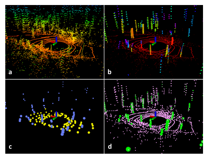
Fig. 2: Feature extraction process for a scan in noisy environment. The original point cloud is shown in (a). In (b), the red points are labeled as ground points. The rest of the points are the points that remain after segmentation. In ©, blue and yellow points indicate edge and planar features in
F
e
F_{e}
Fe and
F
p
F_{p}
Fp. In (d), the green and pink points represent edge and planar features in
F
e
\mathbb{F}_{e}
Fe and
F
p
\mathbb{F}_{p}
Fp respectively.
图2:噪声环境中扫描的特征提取过程。原始点云如(a)所示。在(b)中,红色点标记为地面点。其余的点是分割后保留的点。在(c)中,蓝色和黄色点表示
F
e
F{e}
Fe和
F
p
F{p}
Fp中的边缘和平面特征。在(d)中,绿色和粉色点分别代表
F
e
\mathbb{F}{e}
Fe和
F
p
\mathbb{F}{p}
Fp中的边缘和平面特征。
F e \mathbb{F}{e} Fe和 F p \mathbb{F}{p} Fp是所有子图像的所有边缘和平面特征的集合
我们从子图像中的每一行提取最大值为 c c c的 n F c n_{F_{c}} nFc边缘特征,这些特征不属于地面。类似地,我们从子图像中的每一行提取最小值为 c c c的 n F p n_{F_{p}} nFp平面特征,这些特征一定属于地面点定义 F e F_{e} Fe和 F p F_{p} Fp是此过程中所有边和平面特征的集合。在这里,我们有 F e ⊂ F e F_{e}\subset\mathbb{F}_{e} Fe⊂Fe和 F p ⊂ F p F_{p}\subset\mathbb{F}_{p} Fp⊂Fp
After this process, only the points (Fig. 2(b)) that may represent large objects, e.g., tree trunks, and ground points are preserved for further processing. At the same time, only these points are saved in the range image. We also obtain three properties for each point: (1) its label as a ground point or segmented point, (2) its column and row index in the range image, and (3) its range value. These properties will be utilized in the following modules.
在此过程之后,仅保留可能代表大型对象(例如树干)的点(图2(b))和地面点,以供进一步处理。同时,范围图像中仅保存这些点。我们还获得了每个点的三个属性:(1)其作为地面点或分割点的标签,(2)其在范围图像中的列和行索引,以及(3)其范围值。这些属性将在以下模块中使用。
C.Feature Extraction
The feature extraction process is similar to the method used in [20]. However, instead of extracting features from raw point clouds, we extract features from ground points and segmented points. Let
S
S
S be the set of continuous points of
p
i
p_{i}
pi from the same row of the range image. Half of the points in
S
S
S are on either side of
p
i
p_{i}
pi. In this paper, we set
∣
S
∣
|S|
∣S∣ to 10 . Using the range values computed during segmentation, we can evaluate the roughness of point
p
i
p_{i}
pi in
S
S
S,
特征提取过程类似于[20]中使用的方法。然而,我们不是从原始点云中提取特征,而是从地面点和分割后的点中提取特征。设
S
S
S为距离图像同一行的
p
i
p_{i}
pi的连续点集。
S
S
S中的一半点位于
p
i
p_{i}
pi的两侧。在本文中,我们将
∣
S
∣
| S |
∣S∣设置为10。使用分割期间计算的范围值,我们可以评估在
S
S
S中的点
p
i
p_{i}
pi的曲率(roughness)值,
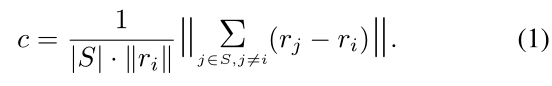
j j j 就是在 i i i 周围的点
曲率 = (当前点到其附近点的距离差 / 当前点的值 ) 的总和再求平均 = 平均的距离差
To evenly extract features from all directions, we divide the range image horizontally into several equal sub-images. Then we sort the points in each row of the sub-image based on their roughness values
c
c
c. Similar to LOAM, we use a threshold
c
t
h
c_{t h}
cth to distinguish different types of features. We call the points with
c
c
c larger than
c
t
h
c_{t h}
cth edge features, and the points with
c
c
c smaller than
c
t
h
c_{t h}
cth planar features. Then
n
F
e
n_{\mathbb{F}_{e}}
nFe edge feature points with the maximum
c
c
c, which do not belong to the ground, are selected from each row in the sub-image.
n
F
p
n_{\mathbb{F}_{p}}
nFp planar feature points with the minimum
c
c
c, which may be labeled as either ground or segmented points, are selected in the same way. Let
F
e
\mathbb{F}_{e}
Fe and
F
p
\mathbb{F}_{p}
Fp be the set of all edge and planar features from all sub-images. These features are visualized in Fig. 2(d). We then extract
n
F
e
n_{F_{e}}
nFe edge features with the maximum
c
c
c, which do not belong to the ground, from each row in the sub-image. Similarly, we extract
n
F
p
n_{F_{p}}
nFp planar features with the minimum
c
c
c, which must be ground points, from each row in the sub-image. Let
F
e
F_{e}
Fe and
F
p
F_{p}
Fp be the set of all edge and planar features from this process. Here, we have
F
e
⊂
F
e
F_{e} \subset \mathbb{F}_{e}
Fe⊂Fe and
F
p
⊂
F
p
.
F_{p} \subset \mathbb{F}_{p} .
Fp⊂Fp. Features in
F
e
F_{e}
Fe and
F
p
F_{p}
Fp are shown in Fig. 2©. In this paper, we divide the
36
0
∘
360^{\circ}
360∘ range image into 6 sub-images. Each sub-image has a resolution of 300 by 16.
n
F
e
,
n
F
p
,
n
F
e
n_{F_{e}}, n_{F_{p}}, n_{\mathbb{F}_{e}}
nFe,nFp,nFe and
n
F
p
n_{\mathbb{F}_{p}}
nFp are chosen to be 2,4 , 40 and 80 respectively.
为了从各个方向均匀地提取特征,我们将距离图像水平分割为几个相等的子图像。然后,我们根据roughness值
c
c
c对子图像每行中的点进行排序。与loam类似,我们使用阈值
c
t
h
c_{t h}
cth来区分不同类型的特征。我们将
c
c
c大于
c
t
h
c_{t h}
cth的点称为边特征点,将
c
c
c小于
c
t
h
c_{t h}
cth平的点称为面特征点。然后,从子图像的每一行中选择最大值为
c
c
c的
n
F
e
n_{\mathbb{F}{e}}
nFe边缘特征点。
n
F
p
n_{\mathbb{F}_{p}}
nFp中具有最小值
c
c
c的平面特征点(可标记为地面点或分段点)的选择方式相同。设
F
e
\mathbb{F}{e}
Fe和
F
p
\mathbb{F}{p}
Fp是所有子图像的所有边缘和平面特征的集合。这些特征如图2(d)所示。然后,我们从子图像中的每一行提取最大值为
c
c
c的
n
F
c
n_{F_{c}}
nFc边缘特征,这些特征不属于地面。类似地,我们从子图像中的每一行提取最小值为
c
c
c的
n
F
p
n_{F_{p}}
nFp平面特征,这些特征一定属于地面点。定义
F
e
F_{e}
Fe和
F
p
F_{p}
Fp是此过程中所有边和平面特征的集合。在这里,我们有
F
e
⊂
F
e
F_{e}\subset\mathbb{F}_{e}
Fe⊂Fe和
F
p
⊂
F
p
F_{p}\subset\mathbb{F}_{p}
Fp⊂Fp。图2(c)显示了
F
e
F_{e}
Fe和
F
p
F_{p}
Fp中的特征。在本文中,我们将
36
0
∘
360^{\circ}
360∘范围图像分为6个子图像。每个子图像的分辨率为300×16线(1800/6 = 300)。
n
F
e
、
n
F
p
n_{F_{e}}、n_{F_{p}}
nFe、nFp(明显的角点和面点)
、
n
F
e
、n_{\mathbb{F}_{e}}
、nFe和
n
F
p
n_{\mathbb{F}_{p}}
nFp分别被选取为2、4、40和80。
D. Lidar Odometry
The lidar odometry module estimates the sensor motion between two consecutive scans. The transformation between two scans is found by performing point-to-edge and pointto-plane scan-matching. In other words, we need to find the corresponding features for points in
F
e
t
F_{e}^{t}
Fet and
F
p
t
F_{p}^{t}
Fpt from feature sets
F
e
t
−
1
\mathbb{F}_{e}^{t-1}
Fet−1 and
F
p
t
−
1
\mathbb{F}_{p}^{t-1}
Fpt−1 of the previous scan. For the sake of brevity, the detailed procedures of finding these correspondences can be found in [20].
激光雷达里程计模块估计两次连续扫描之间的传感器运动。通过执行点到边和点到平面扫描匹配,可以找到两次扫描之间的转换。换句话说,我们需要从上一次扫描的特征集
F
e
t
−
1
\mathbb{F}_{e}^{t-1}
Fet−1和
F
p
t
−
1
\mathbb{F}_{p}^{t-1}
Fpt−1中找到
F
e
t
F_{e}^{t}
Fet 和
F
p
t
F_{p}^{t}
Fpt中的点的相应特征。为简洁起见,可在[20]中找到查找这些对应关系的详细程序。
However, we note that a few changes can be made to improve feature matching accuracy and efficiency:
但是,我们注意到,可以进行一些更改以提高特征匹配的准确性和效率:
(1) Label Matching: Since each feature in
F
e
t
F_{e}^{t}
Fet and
F
p
t
F_{p}^{t}
Fpt is encoded with its label after segmentation, we only find correspondences that have the same label from
F
e
t
−
1
\mathbb{F}_{e}^{t-1}
Fet−1 and
F
p
t
−
1
\mathbb{F}_{p}^{t-1}
Fpt−1. For planar features in
F
p
t
F_{p}^{t}
Fpt, only points that are labeled as ground points in
F
p
t
−
1
\mathbb{F}_{p}^{t-1}
Fpt−1 are used for finding a planar patch as the correspondence. For an edge feature in
F
e
t
F_{e}^{t}
Fet, its corresponding edge line is found in the
F
e
t
−
1
\mathbb{F}_{e}^{t-1}
Fet−1 from segmented clusters. Finding the correspondences in this way can help improve the matching accuracy. In other words, the matching correspondences for the same object are more likely to be found between two scans. This process also narrows down the potential candidates for correspondences.
(1)基于标签的匹配:由于
F
e
t
F_{e}^{t}
Fet和
F
p
t
F_{p}^{t}
Fpt中的每个特征在聚类后都使用标签进行编码,因此我们只能从
F
e
t
−
1
\mathbb{F}_{e}^{t-1}
Fet−1 和
F
p
t
−
1
\mathbb{F}_{p}^{t-1}
Fpt−1中找到具有相同标签的对应关系。对于
F
p
t
F_{p}^{t}
Fpt中的平面要素,仅使用在
F
p
t
−
1
\mathbb{F}_{p}^{t-1}
Fpt−1中标记为地面点的点用于查找planar patch作为对应。对于
F
e
t
F_{e}^{t}
Fet中的边特征,其对应的边线位于分段簇的
F
e
t
−
1
\mathbb{F}_{e}^{t-1}
Fet−1中。用这种方法寻找对应关系有助于提高匹配精度。换句话说,同一对象的匹配对应更可能在两次扫描之间找到。这一过程也缩小了潜在匹配对象的范围。
(2) Two-step L-M Optimization: In [20], a series of nonlinear expressions for the distances between the edge and planar feature points from the current scan and their correspondences from the previous scan are compiled into a single comprehensive distance vector. The Levenberg-Marquardt (L-M) method is applied to find the minimum-distance transformation between the two consecutive scans.
(2) 两步L-M优化:在[20]中,将当前扫描的边缘和平面特征点之间的距离及其与前一次扫描的对应关系的一系列非线性表达式编译成一个综合距离向量。采用Levenberg-Marquardt(L-M)方法来寻找最小距离两次连续扫描之间的转换。
We introduce a two-step L-M optimization method here. The optimal transformation
T
T
T is found in two steps: (1)
[
t
z
,
θ
roll
,
θ
pitch
]
\left[t_{z}, \theta_{\text {roll }}, \theta_{\text {pitch }}\right]
[tz,θroll ,θpitch ] are estimated by matching the planar features in
F
p
t
F_{p}^{t}
Fpt and their correspondences in
F
p
t
−
1
\mathbb{F}_{p}^{t-1}
Fpt−1, (2) the remaining
[
t
x
,
t
y
,
θ
yaw
]
\left[t_{x}, t_{y}, \theta_{\text {yaw }}\right]
[tx,ty,θyaw ] are then estimated using the edge features in
F
e
t
F_{e}^{t}
Fet and their correspondences in
F
e
t
−
1
\mathbb{F}_{e}^{t-1}
Fet−1 while using
[
t
z
,
θ
roll
,
θ
pitch
]
\left[t_{z}, \theta_{\text {roll }}, \theta_{\text {pitch }}\right]
[tz,θroll ,θpitch ] as constraints. It should be noted that though
[
t
x
,
t
y
,
θ
y
a
w
]
\left[t_{x}, t_{y}, \theta_{y a w}\right]
[tx,ty,θyaw] can also be obtained from the first optimization step, they are less accurate and not used for the second step. Finally, the 6D transformation between two consecutive scans is found by fusing
[
t
z
,
θ
roll
,
θ
pitch
]
\left[t_{z}, \theta_{\text {roll }}, \theta_{\text {pitch }}\right]
[tz,θroll ,θpitch ] and
[
t
x
,
t
y
,
θ
y
a
w
]
\left[t_{x}, t_{y}, \theta_{y a w}\right]
[tx,ty,θyaw]. By using the proposed two-step optimization method, we observe that similar accuracy can be achieved while computation time is reduced by about
35
%
35 \%
35% (Table III).
本文介绍了一种两步L-M优化方法。最佳的变换矩阵
T
T
T由两步计算获得:(1)通过匹配
F
p
t
F_{p}^{t}
Fpt中的平面特征和它们在
F
p
t
−
1
\mathbb{F}_{p}^{t-1}
Fpt−1中的对应关系来估计
[
t
z
,
θ
roll
,
θ
pitch
]
\left[t_{z}, \theta_{\text {roll }}, \theta_{\text {pitch }}\right]
[tz,θroll ,θpitch ],(2)剩余的
[
t
x
,
t
y
,
θ
yaw
]
\left[t_{x}, t_{y}, \theta_{\text {yaw }}\right]
[tx,ty,θyaw ]使用
F
e
t
F_{e}^{t}
Fet 中的边特征和它们在
F
e
t
−
1
\mathbb{F}_{e}^{t-1}
Fet−1中的对应关系来估计,同时使用
[
t
z
,
θ
roll
,
θ
pitch
]
\left[t_{z}, \theta_{\text {roll }}, \theta_{\text {pitch }}\right]
[tz,θroll ,θpitch ]作为约束。应该注意的是,虽然也可以从第一个优化步骤中获得
[
t
x
,
t
y
,
θ
y
a
w
]
\left[t_{x}, t_{y}, \theta_{y a w}\right]
[tx,ty,θyaw],但它们的精度较低,并且不用于第二个步骤。最后,通过融合
[
t
z
,
θ
roll
,
θ
pitch
]
\left[t_{z}, \theta_{\text {roll }}, \theta_{\text {pitch }}\right]
[tz,θroll ,θpitch ] 和
[
t
x
,
t
y
,
θ
y
a
w
]
\left[t_{x}, t_{y}, \theta_{y a w}\right]
[tx,ty,θyaw]找到两个连续扫描之间的6D转换。通过使用提出的两步优化方法,我们观察到,在计算时间减少约
35
%
35\%
35%的情况下,可以达到类似的精度(表III)。
由于第一步针对地面点的优化使用点到面的约束来构建约束,修改点的x,y和yaw角不会对点到面的距离产生影响,所以认为地面点之间的约束对 [ t x , t y , θ yaw ] \left[t_{x}, t_{y}, \theta_{\text {yaw }}\right] [tx,ty,θyaw ]不可观

E. Lidar Mapping
The lidar mapping module matches features in
{
F
e
t
,
F
p
t
}
\left\{\mathbb{F}_{e}^{t}, \mathbb{F}_{p}^{t}\right\}
{Fet,Fpt} to a surrounding point cloud map
Q
ˉ
t
−
1
\bar{Q}^{t-1}
Qˉt−1 to further refine the pose transformation, but runs at a lower frequency. Then the L-M method is used here again to obtain the final transformation. We refer the reader to the description from [20] for the detailed matching and optimization procedure.
激光雷达建图模块将
{
F
e
t
,
F
p
t
}
\left\{\mathbb{F}_{e}^{t}, \mathbb{F}_{p}^{t}\right\}
{Fet,Fpt}中的特征与周围的点云映射
Q
ˉ
t
−
1
\bar{Q}^{t-1}
Qˉt−1进行匹配,以进一步优化姿势变换,但运行频率较低。然后,这里再次使用L-M方法来获得最终转换。我们请读者参考[20]中的描述,了解详细的匹配和优化过程。
The main difference in LeGO-LOAM is how the final point cloud map is stored. Instead of saving a single point cloud map, we save each individual feature set
{
F
e
t
,
F
p
t
}
\left\{\mathbb{F}_{e}^{t}, \mathbb{F}_{p}^{t}\right\}
{Fet,Fpt}. Let
M
t
−
1
=
{
{
F
e
1
,
F
p
1
}
,
…
,
{
F
e
t
−
1
,
F
p
t
−
1
}
}
M^{t-1}=\left\{\left\{\mathbb{F}_{e}^{1}, \mathbb{F}_{p}^{1}\right\}, \ldots,\left\{\mathbb{F}_{e}^{t-1}, \mathbb{F}_{p}^{t-1}\right\}\right\}
Mt−1={{Fe1,Fp1},…,{Fet−1,Fpt−1}} be the set that saves all previous feature sets. Each feature set in
M
t
−
1
M^{t-1}
Mt−1 is also associated with the pose of the sensor when the scan is taken. Then
Q
ˉ
t
−
1
\bar{Q}^{t-1}
Qˉt−1 can be obtained from
M
t
−
1
M^{t-1}
Mt−1 in two ways.
LeGO-LOAM的主要区别在于最终点云地图的存储方式。我们不保存单个点云地图,而是保存每个单独的特征集
{
F
e
t
,
F
p
t
}
\left\{\mathbb{F}_{e}^{t}, \mathbb{F}_{p}^{t}\right\}
{Fet,Fpt}。定义
M
t
−
1
=
{
{
F
e
1
,
F
p
1
}
,
…
,
{
F
e
t
−
1
,
F
p
t
−
1
}
}
M^{t-1}=\left\{\left\{\mathbb{F}_{e}^{1}, \mathbb{F}_{p}^{1}\right\}, \ldots,\left\{\mathbb{F}_{e}^{t-1}, \mathbb{F}_{p}^{t-1}\right\}\right\}
Mt−1={{Fe1,Fp1},…,{Fet−1,Fpt−1}} 为保存所有先前特征的集合。
M
t
−
1
M^{t-1}
Mt−1 中的每个特征集也与扫描时传感器的姿势对应。然后
Q
ˉ
t
−
1
\bar{Q}^{t-1}
Qˉt−1可以通过两种方式从
M
t
−
1
M^{t-1}
Mt−1获得。
In the first approach,
Q
ˉ
t
−
1
\bar{Q}^{t-1}
Qˉt−1 is obtained by choosing the feature sets that are in the field of view of the sensor. For simplicity, we can choose the feature sets whose sensor poses are within
100
m
100 \mathrm{~m}
100 m of the current position of the sensor. The chosen feature sets are then transformed and fused into a single surrounding map
Q
ˉ
t
−
1
\bar{Q}^{t-1}
Qˉt−1. This map selection technique is similar to the method used in [20].
在第一种方法中,
Q
ˉ
t
−
1
\bar{Q}^{t-1}
Qˉt−1是通过选择传感器视野中的特征集获得的。为简单起见,我们可以选择传感器位姿在传感器当前位置
100
m
100\mathrm{~m}
100 m范围内的特征集(离当前帧小于100m的关键帧)。然后,将所选的特征集转换并融合为单个局部地图
Q
ˉ
t
−
1
\bar{Q}^{t-1}
Qˉt−1(将关键帧拼起来获得一个局部地图)。这种地图选择技术类似于[20]中使用的方法。
We can also integrate pose-graph SLAM into LeGOLOAM. The sensor pose of each feature set can be modeled as a node in a pose graph. Feature set
{
F
e
t
,
F
p
t
}
\left\{\mathbb{F}_{e}^{t}, \mathbb{F}_{p}^{t}\right\}
{Fet,Fpt} can be viewed as a sensor measurement of this node. Since the pose estimation drift of the lidar mapping module is very low, we can assume that there is no drift over a short period of time. In this way,
Q
ˉ
t
−
1
\bar{Q}^{t-1}
Qˉt−1 can be formed by choosing a recent group of feature sets, i.e.,
Q
ˉ
t
−
1
=
\bar{Q}^{t-1}=
Qˉt−1=
{
{
F
e
t
−
k
,
F
p
t
−
k
}
,
…
,
{
F
e
t
−
1
,
F
p
t
−
1
}
}
\left\{\left\{\mathbb{F}_{e}^{t-k}, \mathbb{F}_{p}^{t-k}\right\}, \ldots,\left\{\mathbb{F}_{e}^{t-1}, \mathbb{F}_{p}^{t-1}\right\}\right\}
{{Fet−k,Fpt−k},…,{Fet−1,Fpt−1}}, where
k
k
k defines the size of
Q
ˉ
t
−
1
\bar{Q}^{t-1}
Qˉt−1. Then, spatial constraints between a new node and the chosen nodes in
Q
ˉ
t
−
1
\bar{Q}^{t-1}
Qˉt−1 can be added using the transformations obtained after L-M optimization. We can further eliminate drift for this module by performing loop closure detection. In this case, new constraints are added if a match is found between the current feature set and a previous feature set using ICP. The estimated pose of the sensor is then updated by sending the pose graph to an optimization system such as [24]. Note that only the experiment in
S
e
c
\mathrm{Sec}
Sec. IV(D) uses this technique to create its surrounding map.
我们还可以将姿势图SLAM集成到LeGOLOAM中。每个特征集的传感器姿势可以建模为姿势图中的一个节点。特征集合集
{
F
e
t
,
F
p
t
}
\left\{\mathbb{F}_{e}^{t}, \mathbb{F}_{p}^{t}\right\}
{Fet,Fpt}可被视为此节点的传感器测量值。由于激光雷达测绘模块的姿态估计漂移非常小,我们可以假设在短时间内没有漂移。在这种方式中,
Q
ˉ
t
−
1
\bar{Q}^{t-1}
Qˉt−1可通过选择最近的一组特征集形成,即
Q
ˉ
t
−
1
=
\bar{Q}^{t-1}=
Qˉt−1=
{
{
F
e
t
−
k
,
F
p
t
−
k
}
,
…
,
{
F
e
t
−
1
,
F
p
t
−
1
}
}
\left\{\left\{\mathbb{F}_{e}^{t-k}, \mathbb{F}_{p}^{t-k}\right\}, \ldots,\left\{\mathbb{F}_{e}^{t-1}, \mathbb{F}_{p}^{t-1}\right\}\right\}
{{Fet−k,Fpt−k},…,{Fet−1,Fpt−1}}, 其中
k
k
k定义
Q
ˉ
t
−
1
\bar{Q}^{t-1}
Qˉt−1的大小。然后,可以使用L-M优化后获得的转换添加
Q
ˉ
t
−
1
\bar{Q}^{t-1}
Qˉt−1中新节点和所选节点之间的空间约束。我们可以通过执行回环检测来进一步消除该模块的漂移。在这种情况下,如果使用ICP在当前特征集和之前的要素集之间找到了匹配项,则会添加新约束。然后,通过将姿势图发送到优化系统(如[24]),更新传感器的估计姿势。请注意,只有
S
e
c
\mathrm{Sec}
Sec.IV(D)中的实验使用此技术创建其周围的地图。
这里的回环比较简单,只要我们在历史的关键帧中找到一帧与当前帧比较近,使用ICP计算两帧的位姿变换,构建一个位姿图模型,来进行一个优化。
IV. Experiment
V. Conclusion
We have proposed LeGO-LOAM, a lightweight and ground-optimized lidar odometry and mapping method, for performing real-time pose estimation of UGVs in complex environments. LeGO-LOAM is lightweight, as it can be used on an embedded system and achieve real-time performance. LeGO-LOAM is also ground-optimized, leveraging ground separation, point cloud segmentation, and improved L-M optimization. Valueless points that may represent unreliable features are filtered out in this process. The two-step L-M optimization computes different components of a pose transformation separately. The proposed method is evaluated on a series of UGV datasets gathered in outdoor environments. The results show that LeGO-LOAM can achieve similar or better accuracy when compared with the state-of-the-art algorithm LOAM. The computation time of LeGO-LOAM is also greatly reduced. Future work involves exploring its application to other classes of vehicles.
我们提出了一种轻量化、基于地面优化的激光雷达里程计和地图绘制方法LeGO LOAM,用于在复杂环境中对UGV进行实时姿态估计。LeGO-LOAM是轻量级的,它可以在嵌入式系统上使用,并实现实时性能。LeGO-LOAM也可以基于地面优化,实现地面分离、点云分割和改进的L-M优化。在此过程中,可能表示不可靠特征的无价值点将被过滤掉。两步L-M优化分别计算姿势变换的不同分量。在室外环境中收集的一系列UGV数据集上对所提出的方法进行了评估。结果表明,与最先进的LOAM算法相比,LeGO LOAM可以达到类似或更好的精度。LeGO-LOAM的计算时间也大大减少。未来的工作包括探索其在其他类别车辆上的应用。
Though LeGO-LOAM is especially optimized for pose estimation on ground vehicles, its application could potentially be extended to other vehicles, e.g., unmanned aerial vehicles (UAVs), with minor changes. When applying LeGO-LOAM to a UAV, we would not assume the ground is present in a scan. A scan’s point cloud would be segmented without ground extraction. The feature extraction process would be the same for the selection of
F
e
,
F
e
F_{e}, \mathbb{F}_{e}
Fe,Fe and
F
p
\mathbb{F}_{p}
Fp. Instead of extracting planar features for
F
p
F_{p}
Fp from points that are labeled as ground points, the features in
F
p
F_{p}
Fp would be selected from all segmented points. Then the original L-M method would be used to obtain the transformation between two scans instead of using the two-step optimization method. Though the computation time will increase after these changes, LeGO-LOAM is still efficient, as a large number of points are omitted in noisy outdoor environments after segmentation. The accuracy of the estimated feature correspondences may improve, as they benefit from segmentation. In addition, the ability to perform loop closures with LeGO-LOAM online makes it a useful tool for long-duration navigation tasks.
尽管 LeGO-LOAM特别适合于地面车辆的姿态估计,但其应用也可以扩展到其他 vehicles,如无人机(UAV),只需稍作改动。当将LeGO-LOAM应用于无人机时,我们不会假设扫描中存在地面。扫描的点云将在不提取地面的情况下进行分割。特征提取过程与选择
F
e
,
F
e
F_{e}, \mathbb{F}_{e}
Fe,Fe 和
F
p
\mathbb{F}_{p}
Fp的过程相同。不再从标记为地面点的点提取
F
p
F_{p}
Fp的平面特征,而是从所有分割点中选择
F
p
F_{p}
Fp中的特征。然后,将使用原始L-M方法来获得两次扫描之间的转换,而不是使用两步优化方法。虽然在这些变化后计算时间会增加,但LeGO-LOAM仍然是有效的,因为分割后在嘈杂的室外环境中忽略了大量的点。估计的特征对应的准确性可能会提高,因为它们受益于分割。此外,LeGO LOAM online执行回环检测的功能使其成为长时间导航任务的有用工具。
相较于LOAM的改进
前端:
- 1.对地面点进行分类和提取,避免一些边缘点的提取
- 2.用了一个简单的点云聚类算法,剔除了一些可能的outlier
后端:
- 1.使用SLAM关键帧的概念对后端部分进行了重构
- 2.引入回环检测和位姿图优化概念,使得地图的全局一致性更好


 1万+
1万+


 被折叠的 条评论
为什么被折叠?
被折叠的 条评论
为什么被折叠?
 到【灌水乐园】发言


