MATLB|和她跌宕起伏最终到达人生之峰【浪漫旅途】

✨🍒🍒🍒🏆🏆🏆😜😜😜🌈🌈🌈💕💕💕💓💓📋📋📋🍺🍺🍺🏅🏅🏅💞💞💞🏆🏆🏆❤️❤️❤️✨✨✨☁️☁️☁️⛅⛅⛅

 

拥有海一样的胸怀，才能有海一样的人生；拥有海一样的宁静，才能镇得住波涛汹涌。做人如海，有跌宕起伏，有波澜不惊。 

💥💥💥💞💞💞欢迎来到本博客❤️❤️❤️💥💥💥

🏆博主优势：🌞🌞🌞博客内容尽量做到思维缜密，逻辑清晰，为了方便读者，方便大家进行学习！亲民！！！还有我开了一个专栏给女朋友的，很浪漫的喔，代码学累的时候去瞧一瞧，看一看：女朋友的浪漫邂逅。有问题可以私密博主，博主看到会在第一时间回复。
 

📋📋📋本文目录如下：⛳️⛳️⛳️

目录

💝漂亮的运行结果 

💝Matlab代码 

 

💝漂亮的运行结果 

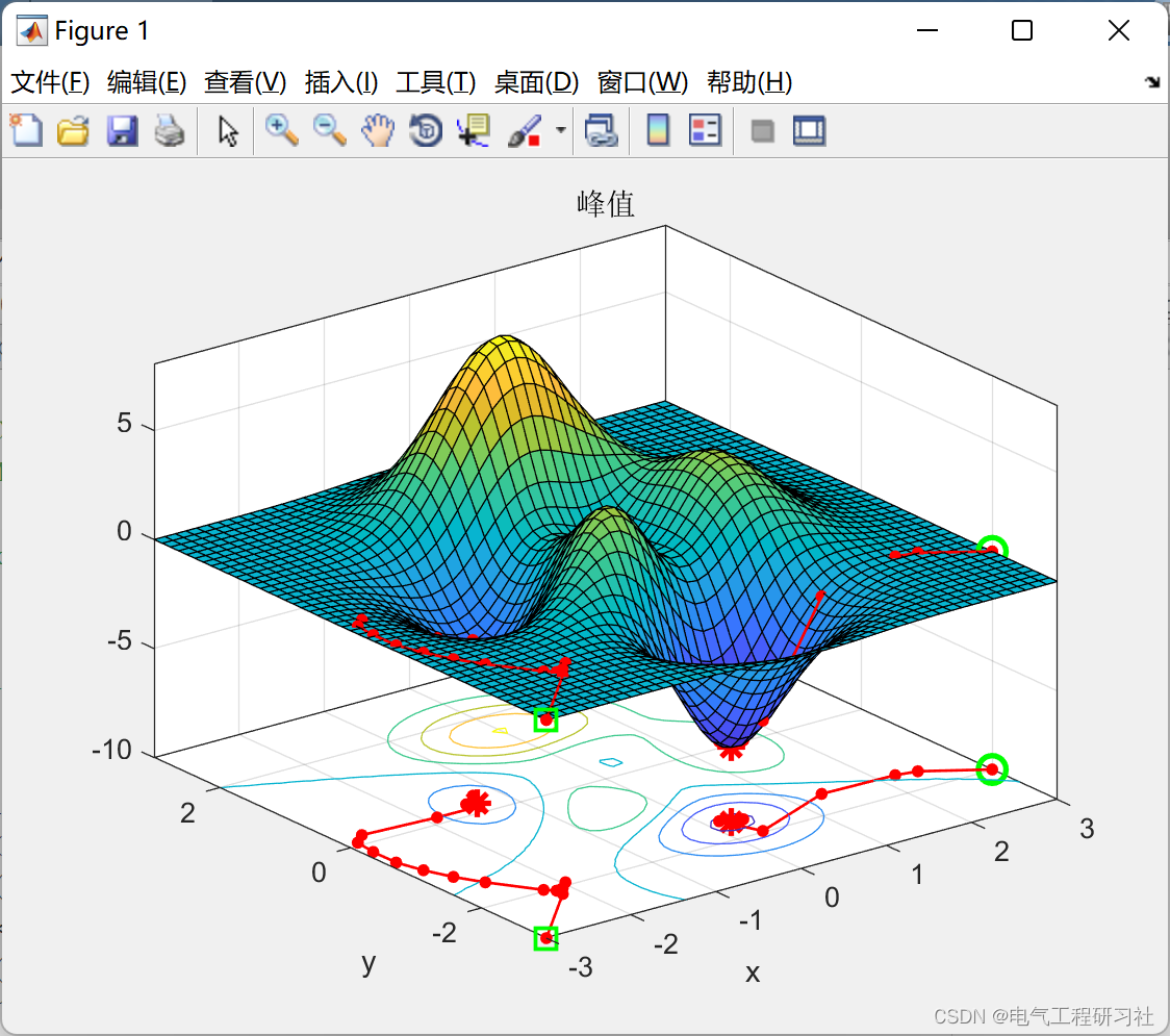
💝Matlab代码 

function [] = LocalMinimaSuffring()

close all; clear all;
global history
history = [];

% *************峰函数****************
dx = 1/8;
[x,y] = meshgrid(-3:dx:3);

z =  3*(1-x).^2.*exp(-(x.^2) - (y+1).^2) ...
   - 10*(x/5 - x.^3 - y.^5).*exp(-x.^2-y.^2) ...
   - 1/3*exp(-(x+1).^2 - y.^2);
 % Self demonstration
  surfc(x,y,z)
  axis('tight')
  xlabel('x'), ylabel('y'), title('峰值')
%% ******************开始********************
x0 = [-3 -3];
y0 = peaksObj(x0);

hold on
plot3(x0(1),x0(2),-10,'gs','lineWidth',2,'MarkerSize',10);
plot3(x0(1),x0(2),y0,'gs','lineWidth',2,'MarkerSize',10);

% [c,ceq] = peaksCon(x0)

options = optimset('Display','iter','OutputFcn',@peaksOutputFcn);
x = fmincon(@peaksObj,x0,[],[],[],[],[],[],@peaksCon,options)

plot3(history(:,1),history(:,2),(-10)*ones(size(history,1)),'-r.','lineWidth',1,'MarkerSize',15)
plot3(history(:,1),history(:,2),history(:,3),'-r.','lineWidth',1,'MarkerSize',15)

plot3(history(end,1),history(end,2),-10,'r*','lineWidth',2,'MarkerSize',10)
plot3(history(end,1),history(end,2),history(end,3),'r*','lineWidth',2,'MarkerSize',10)

%% ******************x0 = [3 -2];********************
history = [];
x0 = [3 -2];

hold on
plot3(x0(1),x0(2),-10,'go','lineWidth',2,'MarkerSize',10);
plot3(x0(1),x0(2),y0,'go','lineWidth',2,'MarkerSize',10);

options = optimset('Display','iter','OutputFcn',@peaksOutputFcn);
x = fmincon(@peaksObj,x0,[],[],[],[],[],[],@peaksCon,options)

plot3(history(:,1),history(:,2),(-10)*ones(size(history,1)),'-r.','lineWidth',1,'MarkerSize',15)
plot3(history(:,1),history(:,2),history(:,3),'-r.','lineWidth',1,'MarkerSize',15)

plot3(history(end,1),history(end,2),-10,'r*','lineWidth',2,'MarkerSize',10)
plot3(history(end,1),history(end,2),history(end,3),'r*','lineWidth',2,'MarkerSize',10)

box on

end  


function stop = peaksOutputFcn(x, optimValues,state)
stop =false;
% hold on;
% plot3(x(1),x(2),-10,'*');
record(x,optimValues.fval);

end

function []=record(x,y)
global history
history=[history;[x,y]]
end

function f = peaksObj(x)
%PEAKSOBJ casts PEAKS function to a form accepted by optimization solvers.
%   PEAKSOBJ(X) calls PEAKS for use as an objective function for an
%   optimization solver.  X must conform to a M x 2 or N x 2 array to be
%   valid input.
%
%   Syntax
%      f = peaksObj(x)
%
%   Example
%      x = [ -3:1:3; -3:1:3]
%      f = peaksObj(x)
%
%   See also peaks

% Check x size to pass data correctly to PEAKS
[m,n] = size(x);

if (m*n) < 2
    error('peaksObj:inputMissing','Not enough inputs');
elseif (m*n) > 2 && (min(m,n) == 1) || (min(m,n) > 2)
    error('peaksObj:inputError','Input must have dimension m x 2');
elseif n ~= 2
    x = x';
end 

% Objective function
f = peaks(x(:,1),x(:,2));
end


function [c,ceq] = peaksCon(x)
%PEAKSCON Constraint function for optimization with PEAKSOBJ
%   PEAKSCON(X) is the constraint function for use with PEAKSOBJ.  X is of
%   size M x 2 or 2 x N.
%
%   Sytnax
%      [c,ceq] = peaksCon(x)
%
%   See also peaksobj, peaks

% Check x size to pass data correctly to constraint definition
[m,n] = size(x);
if (m*n) < 2
    error('peaksObj:inputMissing','Not enough inputs');
elseif (m*n) > 2 && (min(m,n) == 1) || (min(m,n) > 2)
    error('peaksObj:inputError','Input must have dimension m x 2');
elseif n ~= 2
    x = x';
end
% Set plot function to plot constraint boundary
try
    mypref = 'peaksNonlinearPlot';
    if ~ispref(mypref)
        addpref(mypref,'doplot',true);
    else
        setpref(mypref,'doplot',true);
    end
catch
end

% Define nonlinear equality constraint
ceq = [];

% Define nonlinear inequality constraint
% x1^2 + x^2 <= 3^2
c = x(:,1).^2 + x(:,2).^2 - 9; 
% fmincon accepted input form is ceq <= 0
end