数据驱动的自适应线性调频模式分解研究（Matlab代码实现）

 👨‍🎓个人主页：研学社的博客  

💥💥💞💞欢迎来到本博客❤️❤️💥💥

🏆博主优势：🌞🌞🌞博客内容尽量做到思维缜密，逻辑清晰，为了方便读者。

⛳️座右铭：行百里者，半于九十。

📋📋📋本文目录如下：🎁🎁🎁

目录

💥1 概述

📚2 运行结果

2.1 平稳信号

2.2 含噪非平稳信号 

2.3 具有闭合模式的信号 

🎉3 参考文献

🌈4 Matlab代码实现

---

💥1 概述

本文讲解一种数据驱动的时变AM-FM信号自适应信号分解方法，数据驱动的自适应线性调频模式分解及其在非平稳条件下机器故障诊断中的应用，机械系统与信号处理，自适应线性调频模式追踪：算法与应用，非线性线性调频模式分解：一种变分方法。

reproduce some results in the paper: Hongbing Wang, Shiqian Chen, et al. Data-driven adaptive chirp mode decomposition with application to machine fault diagnosis under non-stationary conditions, Mechanical Systems and Signal Processing, 2022. The algorithm used in the paper is an improved version of that in the paper: Shiqian Chen, et al. Adaptive chirp mode pursuit: Algorithm and applications, Mechanical Systems and Signal Processing, 2018. Some of the scripts are adopted from the paper: Shiqian Chen, et al. Nonlinear Chirp Mode Decomposition: A Variational Method, IEEE Transactions on Signal Processing, 2017. and the paper: Shiqian Chen, et al. Detection of rub-impact fault for rotor-stator systems: A novel method based on adaptive chirp mode decomposition, Journal of Sound and Vibration, 2019.

📚2 运行结果

2.1 平稳信号

 

 

 

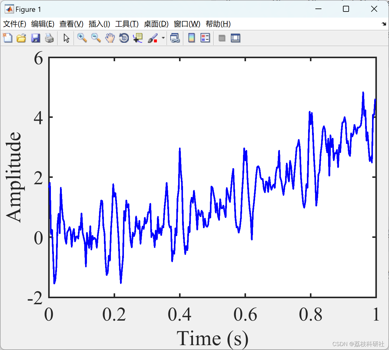
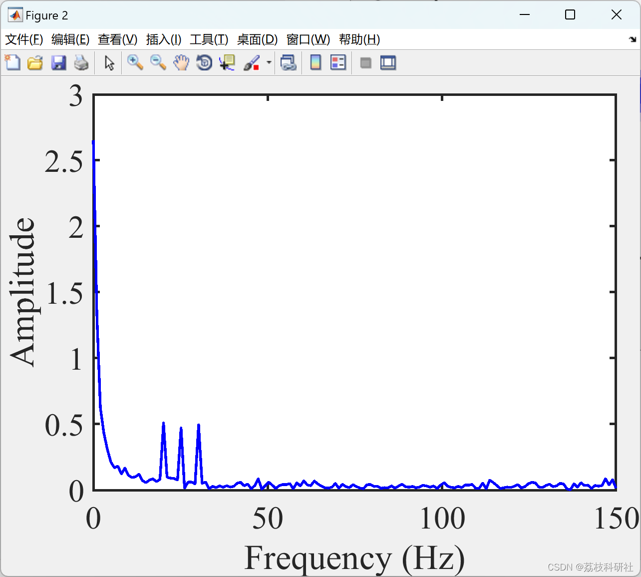
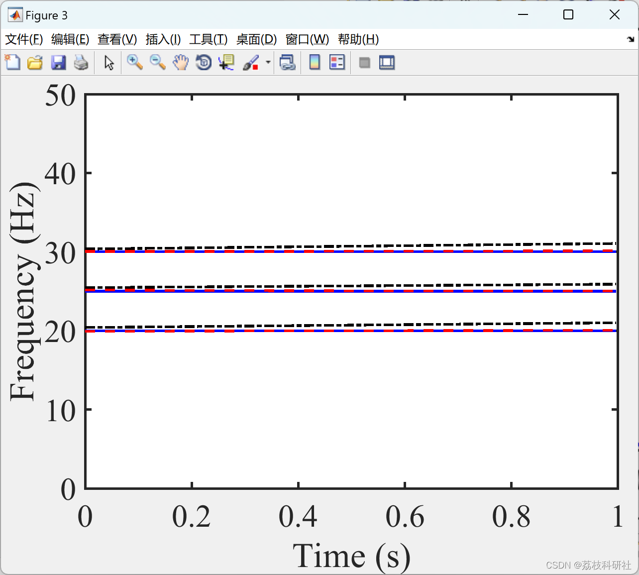
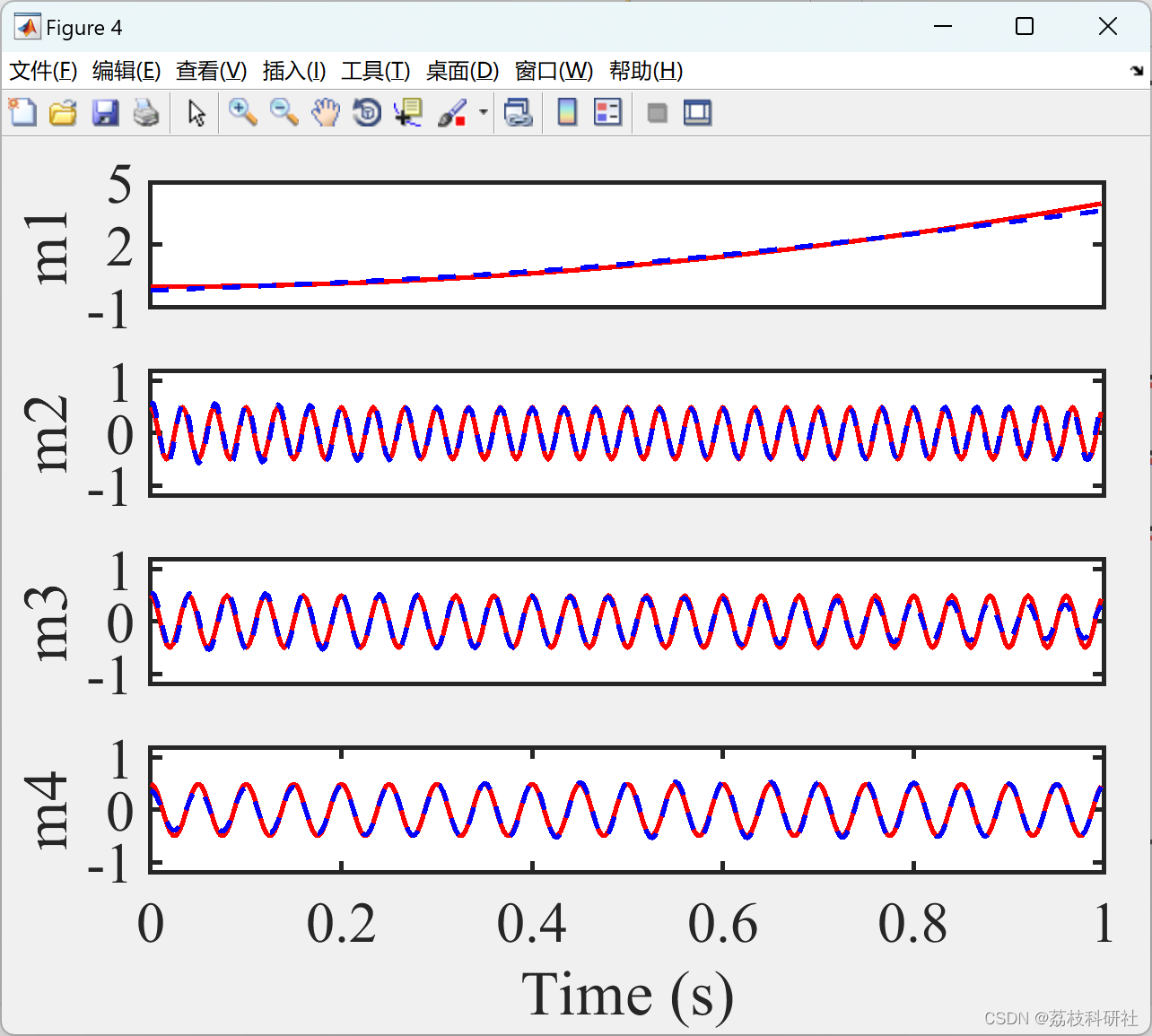
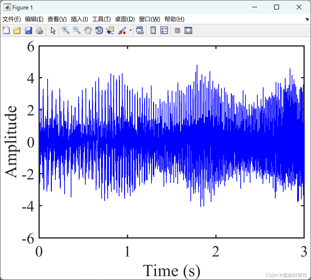
2.2 含噪非平稳信号 

 

 

 

 

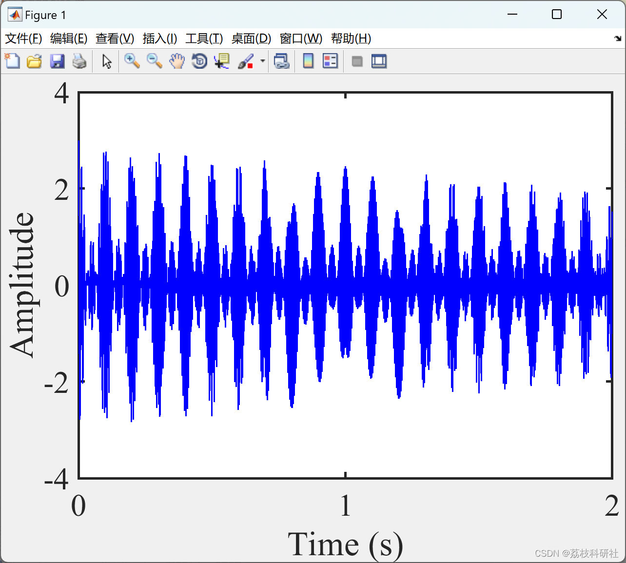
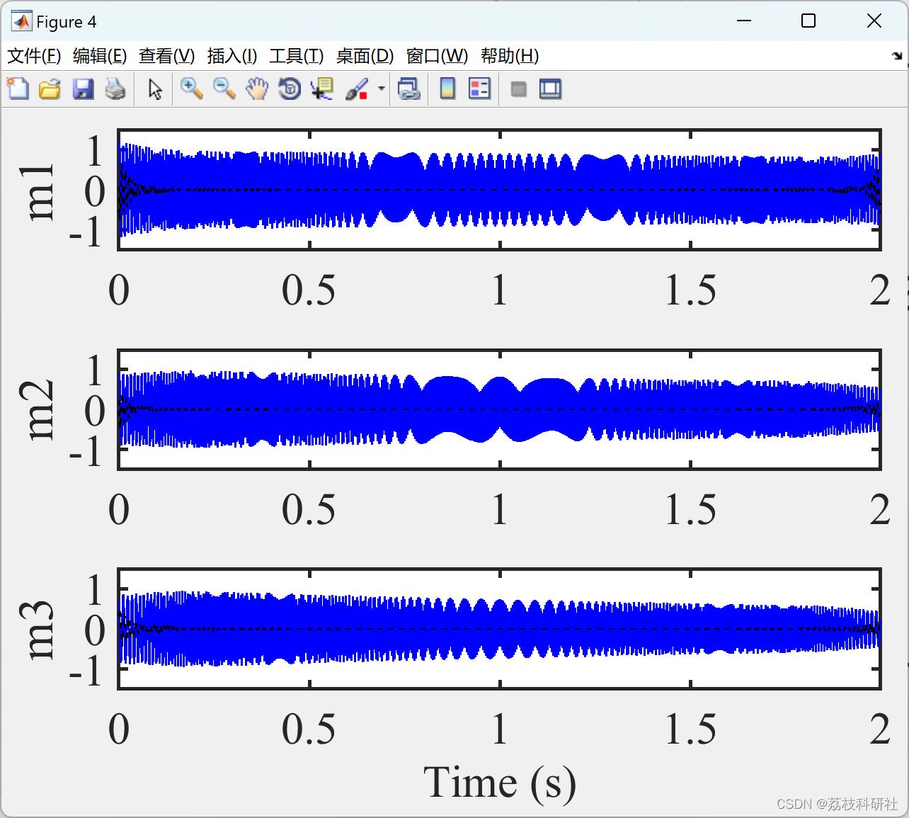
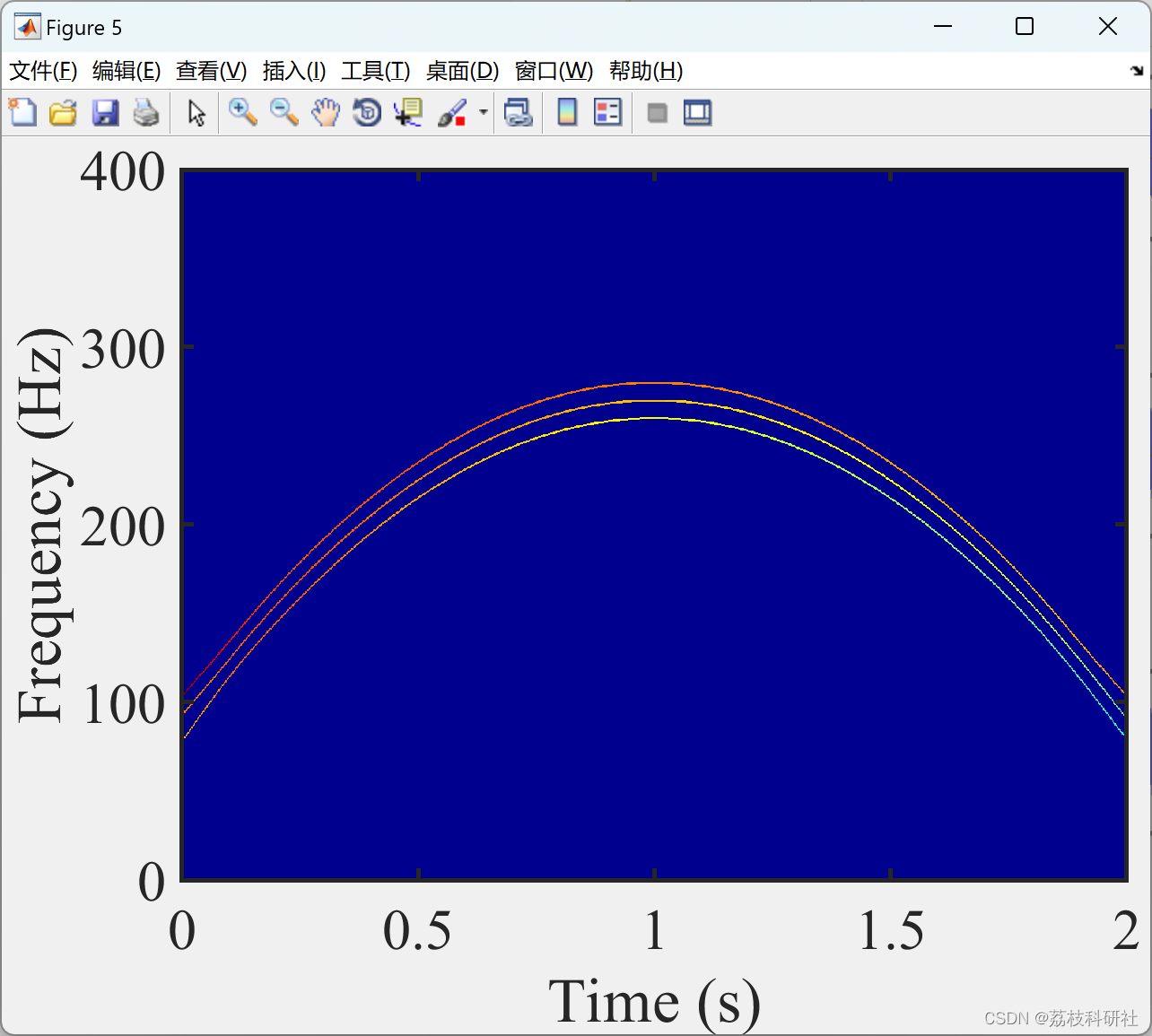
2.3 具有闭合模式的信号 

 

 

 

 

部分代码：

%%%%%%%%% Signal with Close modes %%%%%%%%%
clc;
clear;
close all;
SampFreq = 800;
t = 0:1/SampFreq:2-1/SampFreq;
a1 =exp(-0.1*t); % Instantaneous amplitude (IA) 1
Sig1 = a1.*cos(2*pi*(-60*t.^3+180*t.^2+100*t)); % mode 1
IF1 = -180*t.^2+360*t+100;% instantaneous frequency (IF) 1
a2 =exp(-0.2*t);% IA 2
Sig2 = a2.*cos(2*pi*(-60*t.^3+180*t.^2+90*t)); % mode 2
IF2 = -180*t.^2+360*t+90;% IF 2
a3 =exp(-0.3*t);% IA 3
Sig3 = a3.*cos(2*pi*(-60*t.^3+180*t.^2+80*t)); % mode 3
IF3 = -180*t.^2+360*t+80;% IF 3
Sig = Sig1 + Sig2 + Sig3;
noise = addnoise(length(Sig),0,0);
Sign = Sig+noise; 

figure
set(gcf,'Position',[20 100 640 500]);
plot(t,Sign,'b-','linewidth',1);
axis([0 2 -4 4]);
set(gca,'xtick',[0:1:2]);set(gca,'ytick',[-4:2:4]);
xlabel('Time (s)','FontSize',24);
ylabel('Amplitude','FontSize',24);
set(gca,'FontSize',24,'FontName','Times New Roman','linewidth',2);
set(gca,'looseInset',[0.02 0.02 0.02 0.02])
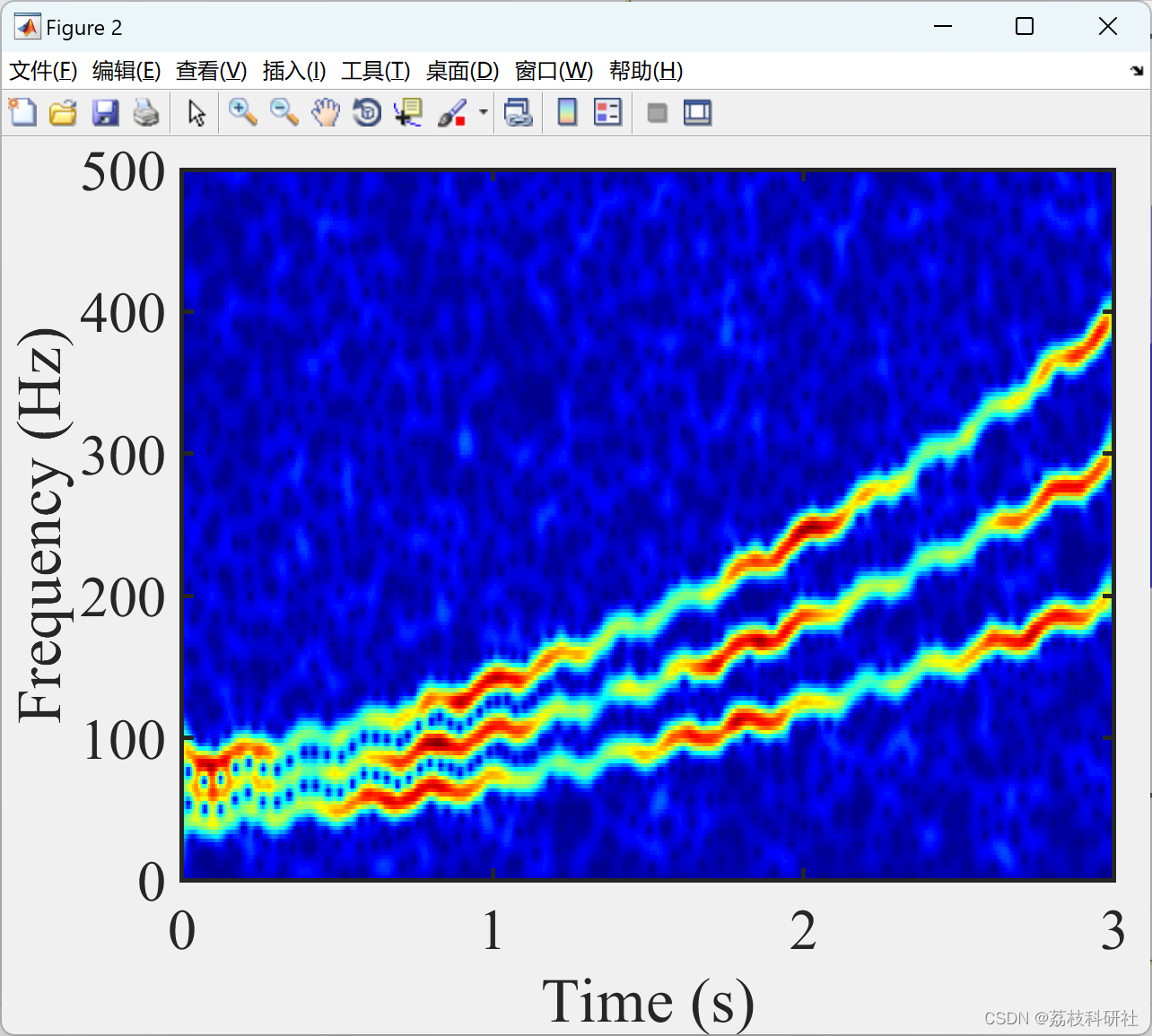
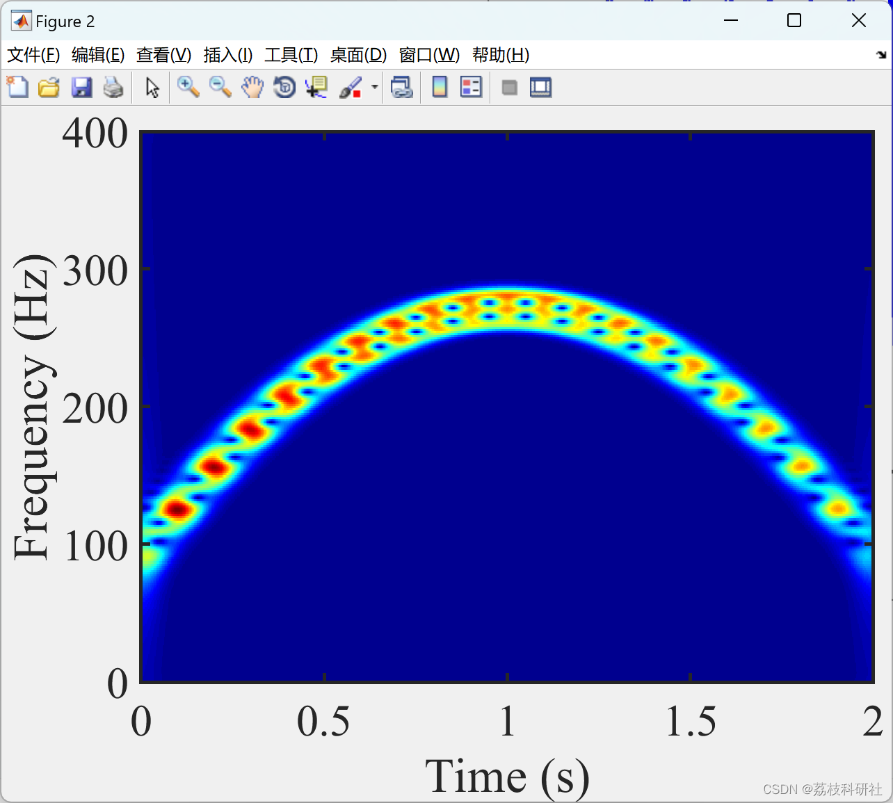
%% Time-frequency distribution (TFD) by STFT
figure
[Spec,f] = STFT(Sign',SampFreq,512,218);
imagesc(t,f,abs(Spec));  
set(gcf,'Position',[20 100 640 500]);    
axis([0 2 0 400]);
xlabel('Time (s)','FontSize',24);
ylabel('Frequency (Hz)','FontSize',24);
set(gca,'YDir','normal');set(gca,'looseInset',[0.02 0.02 0.02 0.02])
set(gca,'FontSize',24,'FontName','Times New Roman','linewidth',2);
colormap('jet')
%% DDACMD
tic
[iniIF,eIF,eIA,IMF] = DDACMD(Sign,SampFreq);
toc
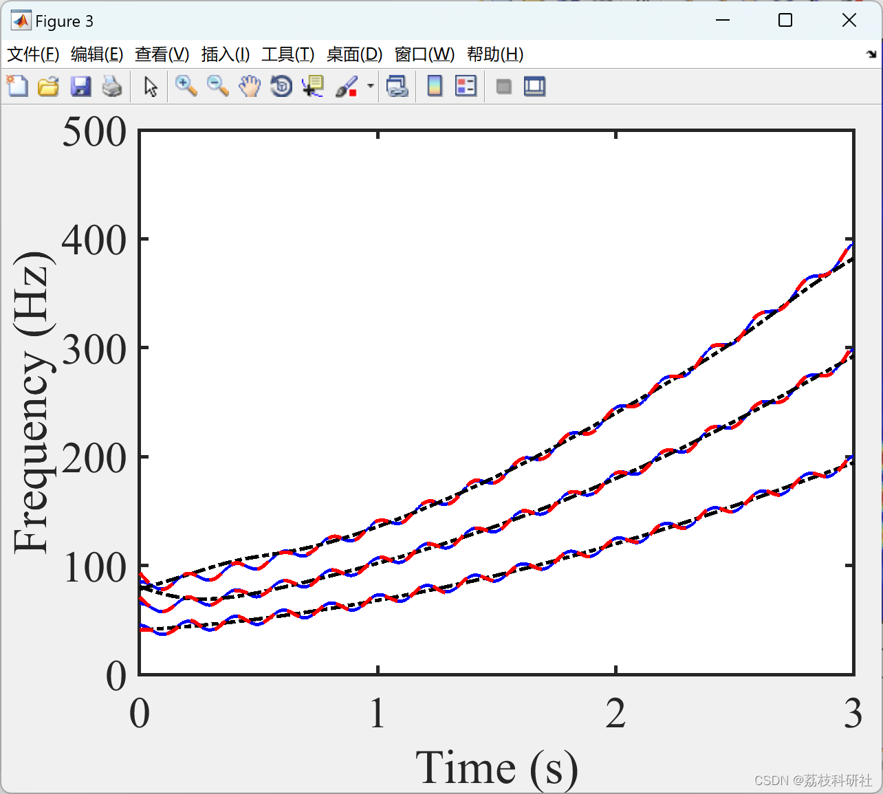
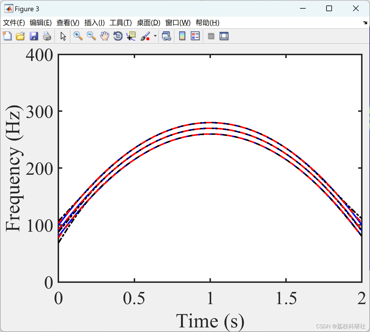
%% Estimated IF
figure
set(gcf,'Position',[20 100 640 500]);
plot(t,IF1,'b-',t,iniIF(1,:),'k-.',t,eIF(1,:),'r--','linewidth',2) 
hold on
plot(t,IF2,'b-',t,iniIF(2,:),'k-.',t,eIF(2,:),'r--','linewidth',2)
hold on
plot(t,IF3,'b-',t,iniIF(3,:),'k-.',t,eIF(3,:),'r--','linewidth',2) 
xlabel('Time (s)','FontSize',24);
ylabel('Frequency (Hz)','FontSize',24);
set(gca,'FontSize',24,'FontName','Times New Roman','linewidth',2);
axis([0 2 0 400]);
set(gca,'looseInset',[0.02 0.02 0.02 0.02])
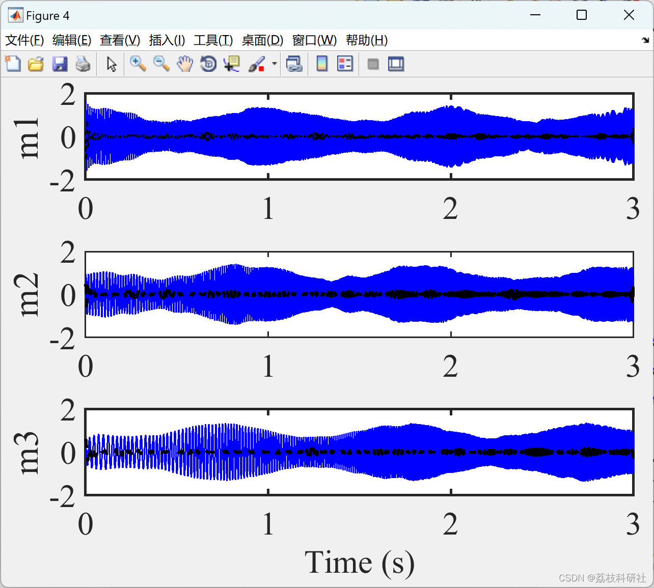
%% Reconstructed modes
figure
set(gcf,'Position',[20 100 640 500]);

axes('position',[0.13 0.80 0.84 0.17]);
plot(t,IMF(1,:),'b-','linewidth',1);
hold on
plot(t,Sig1-IMF(1,:),'k--','MarkerIndices',1:60:length(t),'linewidth',1);
axis([0 2 -1.5 1.5]);set(gca,'xtick',[0:0.5:2]);set(gca,'ytick',[-1 0 1]);
ylabel('m1','FontSize',24);
set(gca,'FontSize',24,'FontName','Times New Roman','linewidth',2);

axes('position',[0.13 0.49 0.84 0.17]);
plot(t,IMF(2,:),'b-','linewidth',1);
hold on
plot(t,Sig2-IMF(2,:),'k--','MarkerIndices',1:60:length(t),'linewidth',1);
axis([0 2 -1.5 1.5]);set(gca,'xtick',[0:0.5:2]);set(gca,'ytick',[-1 0 1]);
ylabel('m2','FontSize',24);
set(gca,'FontSize',24,'FontName','Times New Roman','linewidth',2);

axes('position',[0.13 0.18 0.84 0.17]);
plot(t,IMF(3,:),'b-','linewidth',1);
hold on
plot(t,Sig3-IMF(3,:),'k--','MarkerIndices',1:60:length(t),'linewidth',1);
axis([0 2 -1.5 1.5]);set(gca,'xtick',[0:0.5:2]);set(gca,'ytick',[-1 0 1]);
ylabel('m3','FontSize',24);
set(gca,'FontSize',24,'FontName','Times New Roman','linewidth',2);
xlabel('Time (s)','FontSize',24);
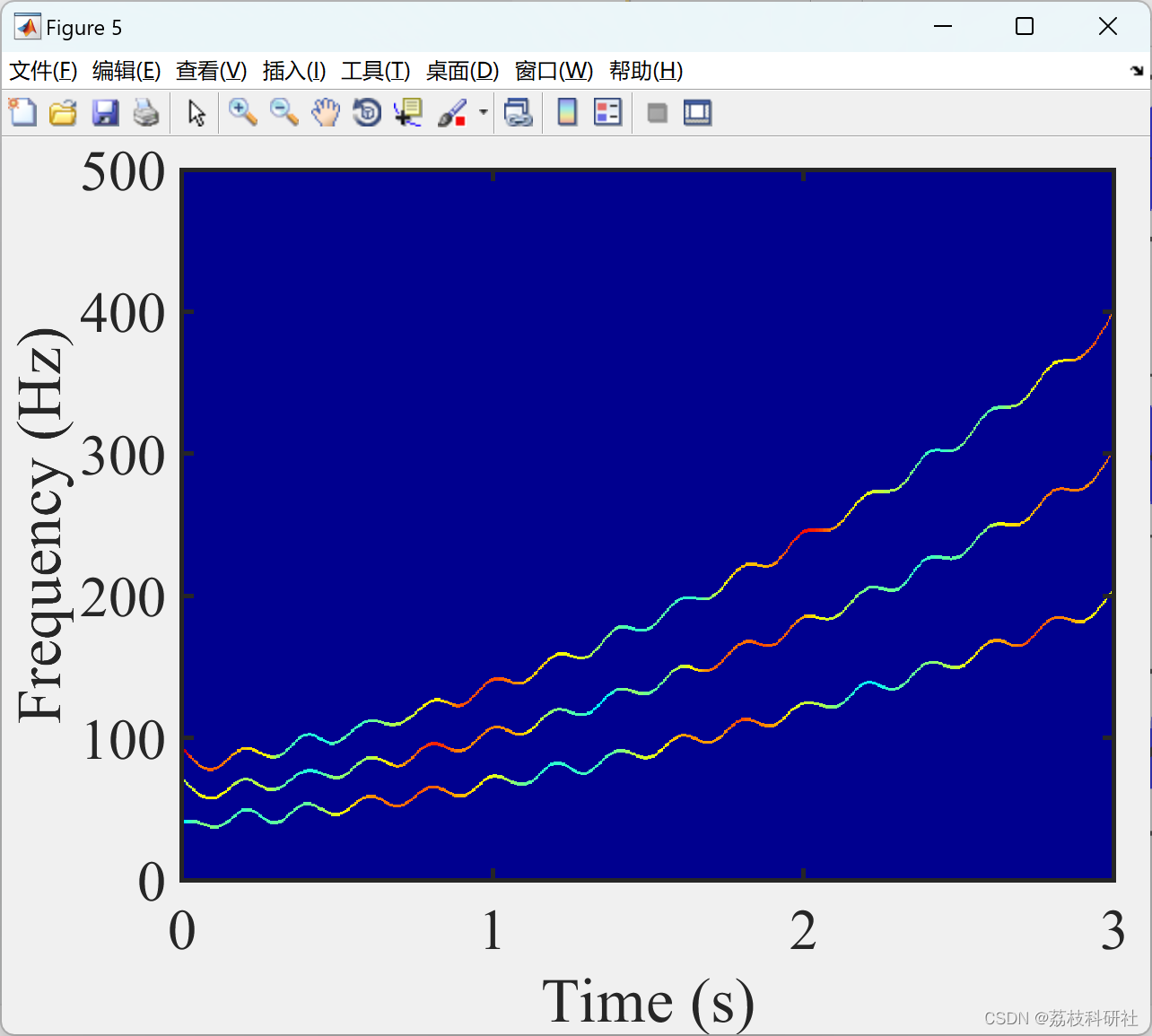
%% Adaptive time-frequency spectrum
band = [0 SampFreq/2];
[ASpec,fbin] = TFspec(eIF(1:3,:),eIA(1:3,:),band);
figure
imagesc(t,fbin,abs(ASpec)); 
set(gcf,'Position',[20 100 640 500]);    
axis([0 2 0 400]);
xlabel('Time (s)','FontSize',24);
ylabel('Frequency (Hz)','FontSize',24);
set(gca,'YDir','normal');set(gca,'looseInset',[0.02 0.02 0.02 0.02])
set(gca,'FontSize',24,'FontName','Times New Roman','linewidth',2);
colormap('jet')

🎉3 参考文献

部分理论来源于网络，如有侵权请联系删除。

[1]陈世谦 （2023）.数据驱动的自适应线性调频模式分解

🌈4 Matlab代码实现