【降低复杂度的双正交匹配追踪（RC-DOMP）算法】无伪逆计算的功率放大器Volterra模型的稀疏识别(Matlab代码实现）

 👨‍🎓个人主页：研学社的博客  

💥💥💞💞欢迎来到本博客❤️❤️💥💥

🏆博主优势：🌞🌞🌞博客内容尽量做到思维缜密，逻辑清晰，为了方便读者。

⛳️座右铭：行百里者，半于九十。

📋📋📋本文目录如下：🎁🎁🎁

目录

💥1 概述

📚2 运行结果

🎉3 参考文献

🌈4 Matlab代码实现

---

💥1 概述

【降低复杂度的双正交匹配追踪（RC-DOMP）算法】无伪逆计算的功率放大器Volterra模型的稀疏识别

📚2 运行结果

 

 

 

 部分代码：

% Load input-output measurement of a 20-MHz 5G-NR at -21 dBm of input power.
load ../data/measurement;

% Load model configuration (Generalized Memory Polynomial (GMP))
modelconfig;

% Generation of signals for identification and validation. Function
% sel_indices selects the indices with the maximum absolute value of the
% output to ensure a proper modeling range. We use 10% of the signal length
% for identification (id) and the complete signal for validation (va). We 
% enable periodic extension (pe) in the validation so the final signal has
% the same length that the measurement.
x = x - mean(x);
y = y - mean(y);

indices = sel_indices(y,0.1);
xid = x(indices);
yid = y(indices);

% model_gmp_generate_X generates the Volterra matrix with the model
% regressors in its columns. Rmat provides a text representation of the
% regressor.
[Xid, yid, Rmat] = model_gmp_generate_X(yid, xid, model);

model.pe = 1
[Xva, yva, Rmat] = model_gmp_generate_X(y, x, model);

% We run the RC-DOMP algorithm for the first Ncoef regressors. Here we analize the whole basis set of 258 coeff.
Ncoef = 258;
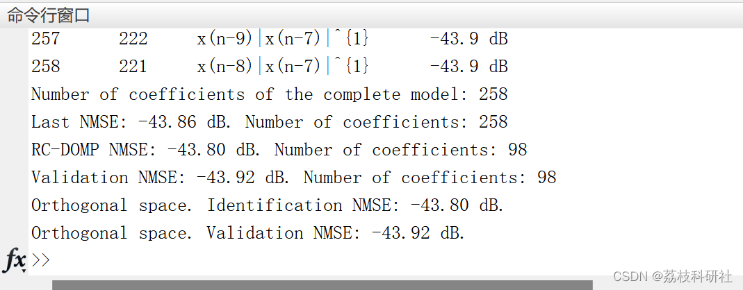
[h, s, nopt, h_full, T] = RCDOMP(Xid, yid, Rmat, Ncoef);

% Validation. Calculation of NMSE.
yest = Xva*h;
nmseva=20*log10(norm(yva-yest,2)/norm(yva,2));
fprintf('Validation NMSE: %4.2f dB. Number of coefficients: %d\n', nmseva, nopt);

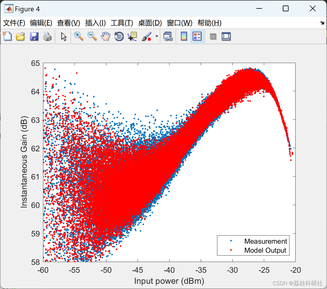
% Plot of the AMAM characteristic of the measurement and the model output.
dBminst = @(x) 10*log10(abs(x).^2/100)+30;
figure, plot(dBminst(x), dBminst(y)-dBminst(x), '.'); xlabel('Input power (dBm)'), ylabel('Instantaneous Gain (dB)');axis([-60 -20 58 65]);
hold on;
plot(dBminst(x), dBminst(yest)-dBminst(x), 'r.');
legend('Measurement','Model Output','Location','Southeast')
saveas(gcf, ['../results/AMAM.png'])

% We get normalized copies of the measurement matrices
Xidnorm = Xid./vecnorm(Xid);
Xvanorm = Xva./vecnorm(Xva);

% Use of matrix T. Z is an orthogonal space. 
% Check Zid(:,i)'*Zid(:,i) = 1
% Check Zid(:,i)'*Zid(:,j) = 0
Zid = Xidnorm*T;
Zva = Xvanorm*T;

% Now the model identification is just a matrix multiplication. We perform
% the estimation with the first nopt regressors in the support set s. 
s = s(1:nopt); % The support set hold the first nopt coefficients
h_orth = Zid(:,s)'*yid; % <-- the pseudoinverse is replaced by Z'

% We traduce the coefficient vector to the Volterra space for using the
% original Volterra matrix to calculate the output. We could also calculate
% the output in the orthogonal space.
h_volterra = diag(vecnorm(Xid(:,s)).^(-1))*T(s,s)*h_orth;

🎉3 参考文献

部分理论来源于网络，如有侵权请联系删除。

[1]J. A. Becerra, M. J. Madero-Ayora, J. Reina-Tosina, C. Crespo-Cadenas (2020) Reduced Complexity Doubly Orthogonal Matching Pursuit (RC-DOMP) 

Title

Sparse Identification of Volterra Models for Power Amplifiers Without Pseudoinverse Computation

Journal/Conference

IEEE Transactions on Microwave Theory and Techniques

🌈4 Matlab代码实现