


💥💥💞💞欢迎来到本博客❤️❤️💥💥
🏆博主优势:🌞🌞🌞博客内容尽量做到思维缜密,逻辑清晰,为了方便读者。
⛳️座右铭:行百里者,半于九十。
📋📋📋本文目录如下:🎁🎁🎁
目录
⛳️赠与读者
👨💻做科研,涉及到一个深在的思想系统,需要科研者逻辑缜密,踏实认真,但是不能只是努力,很多时候借力比努力更重要,然后还要有仰望星空的创新点和启发点。当哲学课上老师问你什么是科学,什么是电的时候,不要觉得这些问题搞笑。哲学是科学之母,哲学就是追究终极问题,寻找那些不言自明只有小孩子会问的但是你却回答不出来的问题。建议读者按目录次序逐一浏览,免得骤然跌入幽暗的迷宫找不到来时的路,它不足为你揭示全部问题的答案,但若能让人胸中升起一朵朵疑云,也未尝不会酿成晚霞斑斓的别一番景致,万一它居然给你带来了一场精神世界的苦雨,那就借机洗刷一下原来存放在那儿的“躺平”上的尘埃吧。
或许,雨过云收,神驰的天地更清朗.......🔎🔎🔎
💥1 概述
【GMSK的最大似然序列检测】采用维特比算法来解决MLSD问题研究
本文包含GMSK的所谓“最大似然序列检测”的常规和快速版本。它采用维特比算法来解决MLSD问题。GMSK的格子结构是减少状态,很值得参考。既有相干接收机,也有非相干接收机。事实上,相干/非相干接收机使用相同的结构,但采用“遗忘因子”方法来产生差异。数学背景以及参考文献可以在项目网站上找到。
有两个测试文件。“GMSK_MLSD_test.m”脚本更直接,更容易理解,它只使用循环来解决维特比算法。“GMSK_MLSD_fast_test.m”采用了一些卷积技巧来减少计算时间,与常规脚本相比,它的速度大约快2倍。
这本质上是一种软输入硬输出类型的维特比算法,因此经过一些修改,它可以很容易地用于任何使用维特比算法的求解器。
【GMSK的最大似然序列检测】采用维特比算法来解决MLSD问题研究
一、引言
GMSK(Gaussian Minimum Shift Keying,高斯最小频移键控)是一种广泛应用于数字通信系统的调制技术。其最大似然序列检测(Maximum Likelihood Sequence Detection,MLSD)是接收端的一种常见解调技术。本文将探讨如何采用维特比算法来解决GMSK的MLSD问题,并介绍相关的数学背景和参考文献。
二、GMSK与MLSD
GMSK调制通过在低速数据流上添加高斯滤波来平滑信号,使得基带信号看起来像是一系列微小的连续相位变化。这种相位变化很小,使得信号接近正弦波形,但又避免了尖锐的切换,从而减少了噪声的影响。MLSD的基本思想是在所有可能的输入序列中找到与接收到的数据最匹配的那个。
三、维特比算法在GMSK MLSD中的应用
维特比算法是一种动态规划算法,特别适用于解决隐马尔可夫模型中的最可能状态序列问题。在GMSK的MLSD中,维特比算法被用来搜索最可能的输入序列,该序列经过GMSK调制后产生的信号与接收到的信号之间的似然比最大。
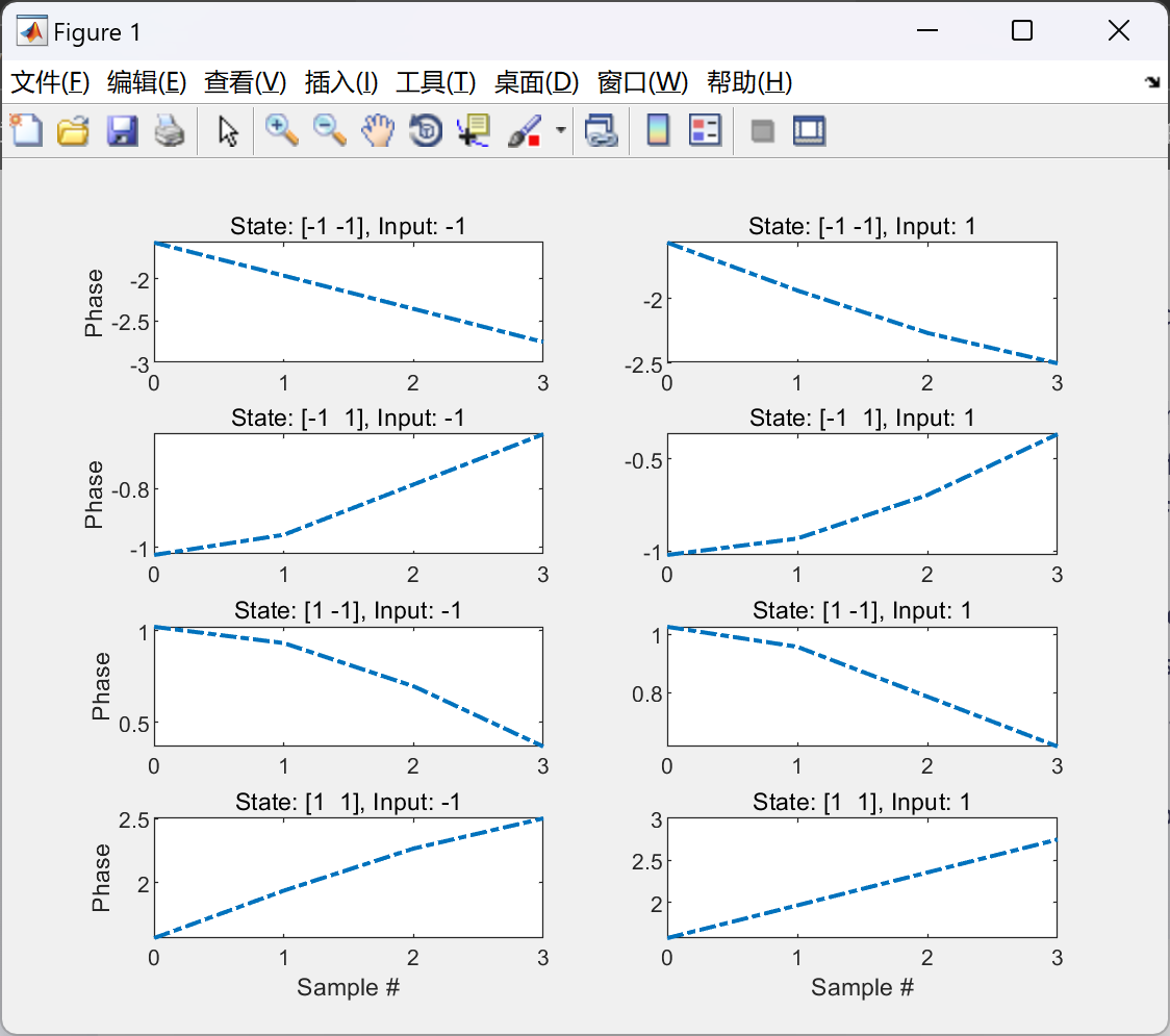
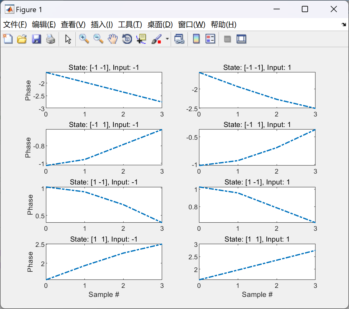
- 格子结构:
- GMSK的格子结构是减少状态的关键。它基于接收到的信号和可能的输入序列之间的相位关系构建。
- 相干接收机和非相干接收机使用相同的格子结构,但采用“遗忘因子”方法来产生差异。遗忘因子用于控制过去状态对当前状态的影响程度。
- 维特比算法的实现:
- 算法初始化时,为格子中的每个状态分配一个初始概率。
- 在每个时间步长中,算法计算从上一个时间步长的每个状态转移到当前状态的所有可能路径的概率。
- 然后,算法选择具有最大概率的路径作为幸存路径,并更新格子中每个状态的概率。
- 最后,算法在达到终止条件时(如达到最大序列长度或格子中的所有状态都被访问过),选择具有最大概率的幸存路径作为最可能的输入序列。
四、测试文件说明
- GMSK_MLSD_test.m:
- 该脚本更直接、更容易理解,它只使用循环来解决维特比算法。
- 它适用于初学者或需要理解维特比算法基本工作原理的人员。
- GMSK_MLSD_fast_test.m:
- 该脚本采用了一些卷积技巧来减少计算时间。
- 与常规脚本相比,它的速度大约快2倍,适用于需要快速处理大量数据的人员。
五、结论
本文介绍了采用维特比算法来解决GMSK的MLSD问题的方法。通过构建GMSK的格子结构和应用维特比算法,可以搜索到最可能的输入序列。同时,本文还提供了两个测试文件来验证算法的正确性和性能。这些研究成果对于优化GMSK调制系统的性能和提高数字通信系统的可靠性具有重要意义。
📚2 运行结果
2.1 GMSK_MLSD_test
2.2 GMSK_MLSD_fast_test

部分代码:
% GMSK Parameters
sps = 4; % oversampling ratio
BT = 0.3; % time bandwidth product
Tsymbol = 1; % symbol interval
modIndex = 0.5; % modulation index (always 0.5 for gmsk)
Tsample = Tsymbol/sps; % sampling interval
L = 3; % Gaussian filter extent
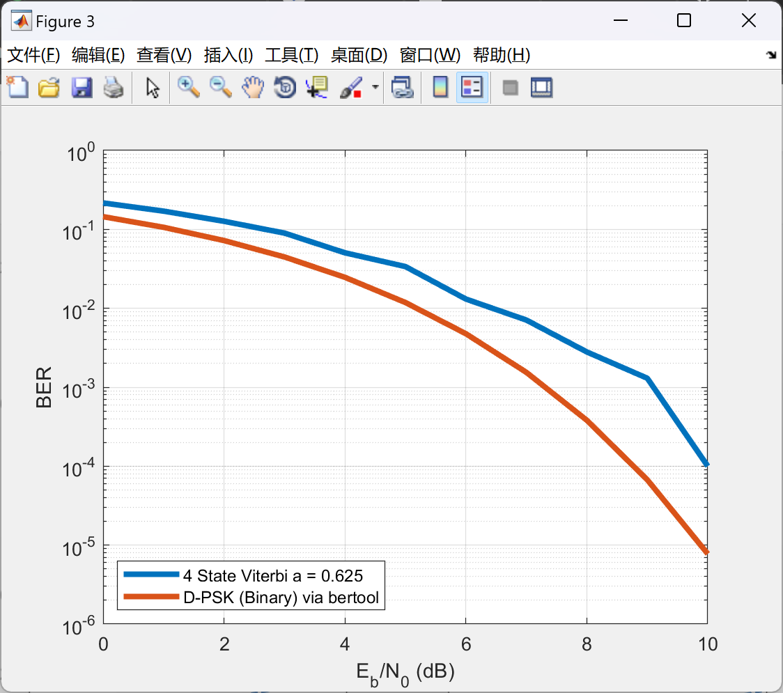
a = 0.625; % forgetting factor for noncoherent MLSD, if a = 1, it solves
% as coherent coherent (a = 1) case should have the same
% performance of D-BPSK
% create the GMSK specific trellis, its actually a small and basic trellis
trellis = gmskTrellis(L);
% generate state bits as 0s and 1s for look up table
state_bits = cell(trellis.numStates, 1);
for state_idx = 1:trellis.numStates
state_bits{state_idx} = de2bi(state_idx-1, L-1, 'left-msb');
end
% branch filter generation for the matched filter
branchFilterCell = branchFilterCellCalc(trellis, L, BT, sps, Tsymbol, modIndex);
% generate data, first L-1 bits of the alpha sequence give the start state
% of the trellis. Start state is actually not so important.
alpha = [zeros(1, L-1), randi([0 1], 1, 1e4)]*2-1; % turn to bipolar NRZ
phi_t = zeros((length(alpha)-(L-1))*sps, 1);
data_idx = 1;
for k=L-1:length(alpha)-1
t = transpose(k*Tsymbol:Tsample:(k+1)*Tsymbol-Tsample); % t is in k*T, (k+1)*T interval
phi_k = sum(alpha(1:k-L+1))*modIndex*pi;
t_mat = bsxfun(@minus, t, (k-L+1:k)*Tsymbol);
g_t = reshape(g_func(t_mat(:), Tsymbol, L, BT)/2, [sps, L]);
phi_t((data_idx-1)*sps+1:data_idx*sps) = phi_k + sum(2*pi*modIndex*bsxfun(@times, g_t, alpha(k-L+2:k+1)), 2);
data_idx = data_idx + 1;
end
init_phase_shift = phi_t(1);
s = exp(1i*phi_t);
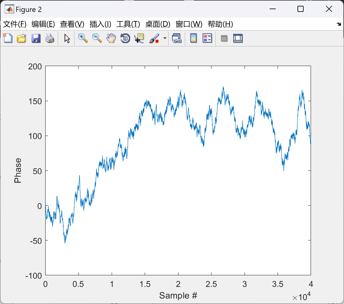
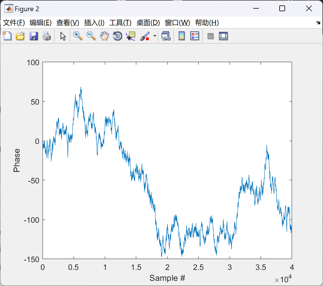
% unwrapped phase of data
figure; plot(unwrap(angle(s)))
xlabel('Sample #'); ylabel('Phase');
snr = [0:10];
Tsymbol = 100e-9; % some symbol duration
Tsample = Tsymbol/sps;
t = (0:length(s)-1)*Tsample; % time vector for the symbol duration
fd=10e3; % some doppler frequence
for snr_no = 1:length(snr)
% multiply s with the commented exponentials to create phase and
% frequency shift if you want to try out noncoherent case
r = awgn(s, snr(snr_no)-10*log10(sps), 'measured'); % *exp(1i*rand*2*pi).*(exp(1i*2*pi*fd*t'))
% Viterbi algorithm start
tic
path_cost = zeros(trellis.numStates, length(alpha)-L+2); % matrix to hold metric results
path = zeros(trellis.numStates, length(alpha)-L+1); % matrix to hold the winner branch state transitions
phase_cost = zeros(trellis.numStates, length(alpha)-L+2); % matrix to hold phase changes due to state transition,
% calculated according to the winner branch
phase_reference = zeros(trellis.numStates, length(alpha)-L+2); % matrix to hold the phase reference, all 1s if coherent
phase_reference(:, 1) = 1; % initialize the first phase reference to 1s
branchCost = zeros(trellis.numStates, 1); % branch metrics
states = unique(trellis.nextStates);
% iterate over all data
for input_idx = L:length(alpha)
input_data = r((input_idx-L)*sps+1:(input_idx-L+1)*sps); % take sps long received signal
% iterate over all end states
for state_idx = 1:trellis.numStates
endState = states(state_idx); % set the end state
% sort of faster branch metric calculation here, we basically
% iterate over all possible start states that reaches the end
% state and calculate their metrics
[row_idx, col_idx] = find(trellis.nextStates == endState); % find the possible start states
z = conv2(input_data, 1, branchFilterCell{state_idx});
z = exp(-1i*phase_cost(row_idx, input_idx-L+1)).*transpose(z(sps, :));
% add the previous winner branch metric to the current branch
% metric for the cumulative path metric then declare the winner
% branch
[branchCost(state_idx), branch_idx] = max(real(z.*conj(phase_reference(row_idx, input_idx-L+1)) ...
+ path_cost(row_idx, input_idx-L+1)));
% find the previous state that corresponds to the winner branch
% and store it in path matrix
previousState_bits = state_bits{row_idx(branch_idx)};
previousState_bits(previousState_bits == 0) = -1;
path(state_idx, input_idx-L+1) = row_idx(branch_idx)-1;
% store the cumulative metric of the winner branch in path cost
% matrix
path_cost(state_idx, input_idx-L+2) = branchCost(state_idx);
% calculate the cumulative phase change that corresponds to the
% winner branch
phase_cost(state_idx, input_idx-L+2) = phase_cost(row_idx(branch_idx), input_idx-L+1) + previousState_bits(1)*pi*modIndex;
% calculate the phase reference of the winner branch according
% to z_vec
phase_reference(state_idx, input_idx-L+2) = a*phase_reference(row_idx(branch_idx), input_idx-L+1) + (1-a)*z(branch_idx);
end
end
🎉3 参考文献
文章中一些内容引自网络,会注明出处或引用为参考文献,难免有未尽之处,如有不妥,请随时联系删除。
[1]张兆晨.自动识别系统(AIS)相干解调技术研究[D].南京理工大学,2012.DOI:10.7666/d.y2062023.
[2]巴少晶.多进制CPM调制在VHF频段高速无线数据传输系统中的均衡技术研究[D].北京邮电大学,2015.
[3]王锋.深空通信GMSK调制体制应用分析和研究[D].湖南大学,2013.
🌈4 Matlab代码实现
资料获取,更多粉丝福利,MATLAB|Simulink|Python资源获取


 466
466

 被折叠的 条评论
为什么被折叠?
被折叠的 条评论
为什么被折叠?
 到【灌水乐园】发言


