图像到图像的映射

图像到图像的映射

1.仿射变换原理

仿射变换的原理就是进行空间的点坐标的变换，官方一点的解释是从二维坐标到二维坐标之间的线性变换，且保持二维图形的“平直性”和“平行性”。其参数公式为

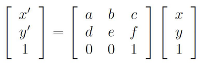
由于仿射变换具有6个自由度，所以需要三个对应点来估计矩阵H。其中X和Y为原坐标，X’和Y’为变换后的坐标，a~f为6个自由度，其中c、f参数分别为x方向和y方向的平移向量。
回到图像扭曲，就是把一个图像的角点映射在另一个图像的某个位置，将其覆盖的像素值替换，合成一幅图像。

代码：

from numpy import *


def normallize(points):
    """在齐次坐标意义下，对点集进行归一化，是最后一行为1"""
    for row in points:
        row /= points[-1]
    return points


def make_homog(points):
    """将点集（dim×n的数组）转换为齐次坐标表示"""

    return vstack((points, ones((1, points.shape[1]))))


def H_from_points(fp, tp):
    """使用线性DLT方法，计算单应性矩阵H，使fp映射到tp。点自动进行归一化"""

    if fp.shape != tp.shape:
        raise RuntimeError('number of points do not match')

    # 对点进行归一化（对数值计算很重要）
    # --- 映射起始点 ---
    m = mean(fp[:2], axis=1)
    maxstd = max(std(fp[:2], axis=1)) + 1e-9
    C1 = diag([1 / maxstd, 1 / maxstd, 1])
    C1[0][2] = -m[0] / maxstd
    C1[1][2] = -m[1] / maxstd
    fp = dot(C1, fp)

    # --- 映射对应点 ---
    m = mean(tp[:2], axis=1)
    maxstd = max(std(tp[:2], axis=1)) + 1e-9
    C2 = diag([1 / maxstd, 1 / maxstd, 1])
    C2[0][2] = -m[0] / maxstd
    C2[1][2] = -m[1] / maxstd
    tp = dot(C2, tp)

    # 创建用于线性方法的矩阵，对于每个对应对，在矩阵中会出现两行数值
    nbr_correspondences = fp.shape[1]
    A = zeros((2 * nbr_correspondences, 9))
    for i in range(nbr_correspondences):
        A[2 * i] = [-fp[0][i], -fp[1][i], -1, 0, 0, 0,
                    tp[0][i] * fp[0][i], tp[0][i] * fp[1][i], tp[0][i]]
        A[2 * i + 1] = [0, 0, 0, -fp[0][i], -fp[1][i], -1,
                        tp[1][i] * fp[0][i], tp[1][i] * fp[1][i], tp[1][i]]

    U, S, V = linalg.svd(A)
    H = V[8].reshape((3, 3))

    # 反归一化
    H = dot(linalg.inv(C2), dot(H, C1))

    # 归一化，然后返回
    return H / H[2, 2]


def Haffine_from_points(fp, tp):
    """计算H仿射变换，使得tp是fp经过仿射变换H得到的"""

    if fp.shape != tp.shape:
        raise RuntimeError('number of points do not match')

    # 对点进行归一化（对数值计算很重要）
    # --- 映射起始点 ---
    m = mean(fp[:2], axis=1)
    maxstd = max(std(fp[:2], axis=1)) + 1e-9
    C1 = diag([1 / maxstd, 1 / maxstd, 1])
    C1[0][2] = -m[0] / maxstd
    C1[1][2] = -m[1] / maxstd
    fp_cond = dot(C1, fp)

    # --- 映射对应点 ---
    m = mean(tp[:2], axis=1)
    C2 = C1.copy()  # 两个点集，必须都进行相同的缩放
    C2[0][2] = -m[0] / maxstd
    C2[1][2] = -m[1] / maxstd
    tp_cond = dot(C2, tp)

    # 因为归一化后点的均值为0，所以平移量为0
    A = concatenate((fp_cond[:2], tp_cond[:2]), axis=0)
    U, S, V = linalg.svd(A.T)

    # 如Hartley和Zisserman著的Multiplr View Geometry In Computer,Scond Edition所示，
    # 创建矩阵B和C
    tmp = V[:2].T
    B = tmp[:2]
    C = tmp[2:4]

    tmp2 = concatenate((dot(C, linalg.pinv(B)), zeros((2, 1))), axis=1)
    H = vstack((tmp2, [0, 0, 1]))

    # 反归一化
    H = dot(linalg.inv(C2), dot(H, C1))

    return H / H[2, 2]

2 .图像扭曲

对图像块应用仿射变换，我们将其称为图像扭曲（或者仿射扭曲）。该操作不仅经常在计算机图形学中，而且经常出现在计算机视觉算法总。扭曲的操作可以使用SciPy工具包中的ndimage包来简单完成。

from numpy import *
from matplotlib.pyplot import *
from scipy import ndimage
from PIL import Image

im = array(Image.open(r'C:\Users\samz305s\Desktop\1.jpg').convert('L'))
H = array([[1.4,0.05,-100],[0.05,1.5,-100],[0,0,1]])
im2 = ndimage.affine_transform(im, H[:2,:2],(H[0,2],H[1,2]))

gray()
subplot(121)
imshow(im)
axis('off')
subplot(122)
imshow(im2)
axis('off')
show()

结果：

3.图中图

from numpy import *
from matplotlib.pyplot import *
from scipy import ndimage
from PIL import Image
import homography


def image_in_image(im1, im2, tp):
    """使用仿射变换将im1放置在im2上，使im1图像的角和tp尽可能的靠近
        tp是齐次表示的，并且是按照从左上角逆时针计算的"""

    # 扭曲的点
    m, n = im1.shape[:2]
    fp = array([[0, m, m, 0], [0, 0, n, n], [1, 1, 1, 1]])

    # 计算仿射变换，并且将其应用于图像im1中
    H = homography.Haffine_from_points(tp, fp)
    im1_t = ndimage.affine_transform(im1, H[:2, :2],
                                     (H[0, 2], H[1, 2]), im2.shape[:2])
    alpha = (im1_t > 0)

    return (1 - alpha) * im2 + alpha * im1_t


im1 = array(Image.open(r'C:\Users\samz305s\Desktop\1.jpg').convert('L'))
im2 = array(Image.open(r'C:\Users\samz305s\Desktop\2.jpg').convert('L'))

gray()
subplot(131)
imshow(im1)
axis('equal')
axis('off')
subplot(132)
imshow(im2)
axis('equal')
axis('off')

# 选定一些目标点
tp = array([[264, 538, 540, 264], [40, 36, 605, 605], [1, 1, 1, 1]])

im3 = image_in_image(im1, im2, tp)
subplot(133)
imshow(im3)
axis('equal')
axis('off')
show()

结果：