单细胞测序数据整合（Seurat V4.0） vignettes

Introduction to scRNA-seq integration • Seurathttps://satijalab.org/seurat/articles/integration_introduction.html

Introduction to scRNA-seq integration

Compiled: January 11, 2022

Source: vignettes/integration_introduction.Rmd

基于R seurat v4.0的内置整合数据方法的R包进行的翻译学习

---

scRNA-seq整合简介

单细胞数据大量产出使得联合分析两个或多个单细胞数据集成为了独特的挑战。特别是在标准工作流下，识别存在于多个数据集中的细胞群可能会有问题。Seurat v4包含一组方法来匹配（或“对齐”）跨数据集的共享细胞群。这些方法首先识别处于匹配生物状态的跨数据集细胞对（“锚定”），既可用于校正数据集之间的技术差异（即批效应校正），也可用于对跨实验条件进行比较性scRNA序列分析。

ps：

锚定：选择相对保守的细胞群，计算样本间的差异成为迁移标准，继而将之用于校正数据集的差异。

下面，我们展示了Stuart*、Butler*等人2019年所述的scRNA-seq整合方法，以对静息状态或干扰素刺激状态下的人类免疫细胞（PBMC）进行比较分析。

---

整合目标

以下教程旨在向您概述使用Seurat整合程序可能对复杂细胞类型进行的比较分析。在这里，我们讨论几个关键目标：

• 构建“整合”数据以进行下游分析
• 确定两个数据集中存在的细胞类型
• 获得在对照细胞和干预细胞中都保守存在的细胞类型标记
• 比较数据集，以找出基于特定细胞类型对刺激所产生的特异性反应

---

设置Seurat对象

为了方便起见，我们使用SeuratData包的ifnb数据集。

library(Seurat)
library(SeuratData)
library(patchwork)

# install dataset
InstallData("ifnb")

# load dataset
LoadData("ifnb")

# split the dataset into a list of two seurat objects (stim and CTRL)
ifnb.list <- SplitObject(ifnb, split.by = "stim")

# normalize and identify variable features for each dataset independently
ifnb.list <- lapply(X = ifnb.list, FUN = function(x) {
    x <- NormalizeData(x)
    x <- FindVariableFeatures(x, selection.method = "vst", nfeatures = 2000)
})

# select features that are repeatedly variable across datasets for integration
features <- SelectIntegrationFeatures(object.list = ifnb.list)

---

执行整合

然后，我们使用FindIntegrationAnchors（）函数识别作为锚的基因，该函数构建一个作为Seurat对象的列表作为输入，并使用这些锚将两个数据集通过IntegratedData（）函数整合在一起。

immune.anchors <- FindIntegrationAnchors(object.list = ifnb.list, anchor.features = features)

# this command creates an 'integrated' data assay
immune.combined <- IntegrateData(anchorset = immune.anchors)

---

进行整合分析

现在我们可以对所有一个细胞文件进行整合分析了！

# specify that we will perform downstream analysis on the corrected data note that the
# original unmodified data still resides in the 'RNA' assay
DefaultAssay(immune.combined) <- "integrated"

# Run the standard workflow for visualization and clustering
immune.combined <- ScaleData(immune.combined, verbose = FALSE)
immune.combined <- RunPCA(immune.combined, npcs = 30, verbose = FALSE)
immune.combined <- RunUMAP(immune.combined, reduction = "pca", dims = 1:30)
immune.combined <- FindNeighbors(immune.combined, reduction = "pca", dims = 1:30)
immune.combined <- FindClusters(immune.combined, resolution = 0.5)

# Visualization
p1 <- DimPlot(immune.combined, reduction = "umap", group.by = "stim")
p2 <- DimPlot(immune.combined, reduction = "umap", label = TRUE, repel = TRUE)
p1 + p2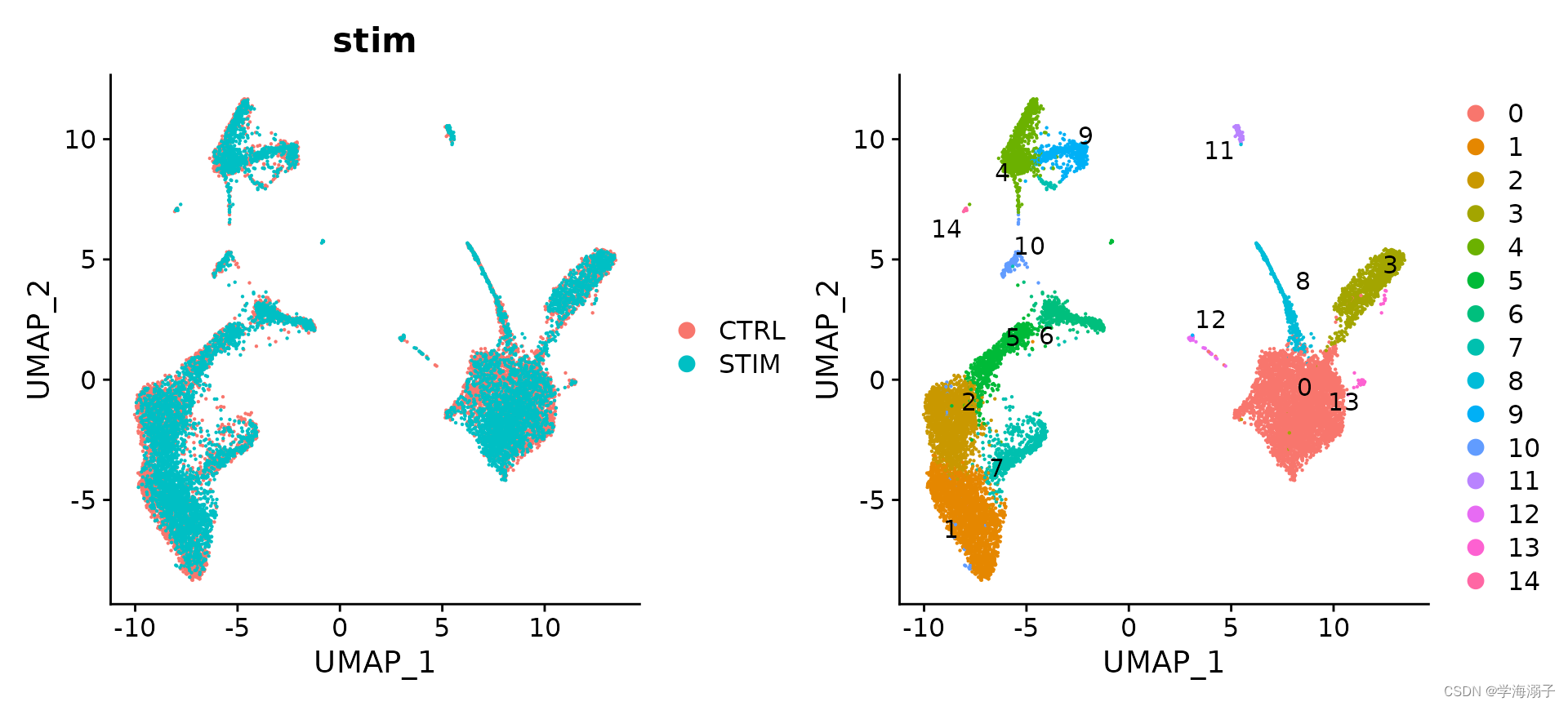

为了将这两种情况并排可视化ÿ