论文阅读：Observation-Centric SORT: Rethinking SORT for Robust Multi-Object Tracking——OC-SORT

大聪聪聪

已于 2023-12-11 17:23:32 修改

阅读量1w

点赞数 15

文章标签：目标跟踪人工智能计算机视觉

于 2022-04-23 10:37:55 首次发布

本文链接：https://blog.csdn.net/weixin_48292639/article/details/124358924

版权

前言

文章的一作是曹金坤，作者同时还是《TransTrack: Multiple Object Tracking with Transformer》的二作。
文章：https://arxiv.org/pdf/2203.14360.pdf
代码：https://github.com/noahcao/OC_SORT
本文为论文阅读记录，本人才疏学浅，应该有错误的认识，希望读者能在评论区帮助我改正错误。
文章提出了一种用于多目标跟踪的算法Obeservation-Centric SORT(OC-SORT),以解决多目标跟踪中模型对目标重叠、非线性运动的敏感和需要高帧率视频的问题。OC-SORT保持了简单、在线、实时的特点，却在目标重叠和非线性运动时具有鲁棒性。
文章检测部分采用的是yolo x，不作过多介绍，我们的重点是作者提出的三种算法。

Introduction

作者回顾了SORT和识别中的三个限制问题，并针对这些问题提出了三种解决算法。

一、3个问题

首先作者回顾了SORT中的三个限制问题：

1估计噪声

虽然检测目标的移动可以近似为线性模型，但是使用高帧率数据增大系统了对状态噪声的敏感性。具体地说，在高帧率视频的连续帧之间，物体位移的噪声可能与实际物体位移的大小相同，就会导致使用卡尔曼滤波器估计物体的速度时存在较大的方差。即用卡尔曼滤波器计算先验估计 $X_{t|t-1}$ 帽时，因为噪音的问题，先验误差协方差矩阵 $P_{t|t-1}$ 特别大，而使得先验估计和真实情况差很远。

2误差积累

由于检测中目标的遮挡或非线性运动，当没有新的检测框与现有轨迹匹配时，对象状态噪声会进一步累积。作者证明了在这种情况下，卡尔曼滤波器对目标位置估计的误差累积是关于时间的平方。例如，MOT17上靠近摄像头的行人大小约为50×300像素。但是，即使假设位置估计的方差在1个像素左右，10帧遮挡也可以将最终位置估计的偏移累积为对象大小的一倍。

3以估计为中心

SORT是以目标估计为中心的，所以非常依赖卡尔曼滤波器的的估计，而检测的结果只作为辅助。但是随着目标检测算法的发展，作者认为检测的结果比卡尔曼滤波器的估计结果更加准确，所以在mot中应该更加以检测为中心。

二、3种解决算法：

1.OOS：Observation-centric Online Smoothing

OOS旨在减少由于检测目标缺少造成的误差积累，在将非活动轨迹与检测到的目标重新关联的框架中，首先为该对象构建一条虚拟轨迹，从跟踪丢失之前的最后一个检测开始，到新匹配到检测结束。沿着这个虚拟轨迹，平滑卡尔曼滤波器参数，以获得更好的目标位置估计。
最后一次观测到的轨迹记录为 $Z_{t1}$ ，再次链接到的轨迹记录为 $Z_{t2}$ ，于是虚拟的轨迹记为：
沿着这个虚拟轨迹，可以从t1时的状态开始，通过在预测阶段，预测等式和协方差 $P_{t|t-1}$ 矩阵：

和更新阶段，卡尔曼增益 $k_{t}$ ，后验估计和更新协方差矩阵 $P_{t|t}$ 更新等式：

来回交替反向检查卡尔曼滤波器的参数，使得误差积累的现象不在发生。
更新的状态估计方程：
更新后验估计
代码：

    def unfreeze(self):
        if self.attr_saved is not None:
            new_history = deepcopy(self.history_obs)#拷贝之前的轨迹
            self.__dict__ = self.attr_saved#更改状态
            # self.history_obs = new_history 
            self.history_obs = self.history_obs[:-1]
            occur = [int(d is None) for d in new_history]
            indices = np.where(np.array(occur)==0)[0]
            index1 = indices[-2]#丢失前最后一帧的序号
            index2 = indices[-1]#重新匹配的帧
            box1 = new_history[index1]#丢失前最后一帧的（x,y,s,r)（x,y)为box中心坐标，s为面积，r为w/h
            x1, y1, s1, r1 = box1 
            w1 = np.sqrt(s1 * r1)
            h1 = np.sqrt(s1 / r1)
            box2 = new_history[index2]#重新匹配的box
            x2, y2, s2, r2 = box2 
            w2 = np.sqrt(s2 * r2)
            h2 = np.sqrt(s2 / r2)
            time_gap = index2 - index1#丢失的帧数
            dx = (x2-x1)/time_gap#两帧之间的x坐标的差
            dy = (y2-y1)/time_gap 
            dw = (w2-w1)/time_gap 
            dh = (h2-h1)/time_gap#同上
            for i in range(index2 - index1):#通过这个for循环模拟更新跟踪过程，减少误差累计
                """
                    The default virtual trajectory generation is by linear
                    motion (constant speed hypothesis), you could modify this 
                    part to implement your own. 
                """
                x = x1 + (i+1) * dx 
                y = y1 + (i+1) * dy 
                w = w1 + (i+1) * dw 
                h = h1 + (i+1) * dh
                s = w * h 
                r = w / float(h)
                new_box = np.array([x, y, s, r]).reshape((4, 1))
                #根据每帧的插值，丢失的第一帧开始模拟历史轨迹
                """
                    I still use predict-update loop here to refresh the parameters,
                    but this can be faster by directly modifying the internal parameters
                    as suggested in the paper. I keep this naive but slow way for 
                    easy read and understanding
                """
                self.update(new_box)#调用卡尔曼滤波器里面的update函数更新后验估计x_post和更新误差协方差P_post 
                if not i == (index2-index1-1):
                    self.predict()#调用trackers/ocsort_tracker/kalmanfilter.py的预测函数得到先验估计x_prior和先验误差协方差p_prior

2.Observation-Centric Momentum(OCM)

线性运动模型假定速度方向一致。然而，由于物体的非线性运动和状态噪声，这种假设往往不成立。但在很短时间内，运动轨迹可以近似为线性，但噪声的存在阻止利用速度方向的一致性。于是作者提出了OCM——一种降低噪声的方法，并将速度一致性（动量）项添加到成本矩阵中。给定N条存在的轨迹和M个检测框，关联成本为：
OCM
伪码： ocm伪代码
速度方向代码：

def speed_direction_batch(dets, tracks):
    tracks = tracks[..., np.newaxis]
    CX1, CY1 = (dets[:,0] + dets[:,2])/2.0, (dets[:,1]+dets[:,3])/2.0
    CX2, CY2 = (tracks[:,0] + tracks[:,2]) /2.0, (tracks[:,1]+tracks[:,3])/2.0
    dx = CX1 - CX2 
    dy = CY1 - CY2 
    norm = np.sqrt(dx**2 + dy**2) + 1e-6
    dx = dx / norm 
    dy = dy / norm
    return dy, dx # size: num_track x num_det

ocm代码：

def associate(detections, trackers, iou_threshold, velocities, previous_obs, vdc_weight):
#vdc_weight=0.2(公式中速度权重)，iou_threhold=0.3(iou阈值，当大于即匹配成功)
    if(len(trackers)==0):
        return np.empty((0,2),dtype=int), np.arange(len(detections)), np.empty((0,5),dtype=int)


    Y, X = speed_direction_batch(detections, previous_obs)

    inertia_Y, inertia_X = velocities[:,0], velocities[:,1]

    inertia_Y = np.repeat(inertia_Y[:, np.newaxis], Y.shape[1], axis=1)
    inertia_X = np.repeat(inertia_X[:, np.newaxis], X.shape[1], axis=1)
    diff_angle_cos = inertia_X * X + inertia_Y * Y
    diff_angle_cos = np.clip(diff_angle_cos, a_min=-1, a_max=1)
    diff_angle = np.arccos(diff_angle_cos)
    diff_angle = (np.pi /2.0 - np.abs(diff_angle)) / np.pi

    valid_mask = np.ones(previous_obs.shape[0])
    valid_mask[np.where(previous_obs[:,4]<0)] = 0

    iou_matrix = shape_iou(detections, trackers)
    scores = np.repeat(detections[:,-1][:, np.newaxis], trackers.shape[0], axis=1)
    # iou_matrix = iou_matrix * scores # a trick sometiems works, we don't encourage this
    valid_mask = np.repeat(valid_mask[:, np.newaxis], X.shape[1], axis=1)

    angle_diff_cost = (valid_mask * diff_angle) * vdc_weight
    angle_diff_cost = angle_diff_cost.T
    angle_diff_cost = angle_diff_cost * scores

    if min(iou_matrix.shape) > 0:
        a = (iou_matrix > iou_threshold).astype(np.int32)
        if a.sum(1).max() == 1 and a.sum(0).max() == 1:
            matched_indices = np.stack(np.where(a), axis=1)
        else:
            matched_indices = linear_assignment(-(iou_matrix+angle_diff_cost))
          #这里在计算COM cost：标准iou cost+速度方向的cost，再通过使用匈牙利算法进行最优匹配

即将速度方向带入到IOU度量矩阵中。X帽为目标的估计状态矩阵， Z为检测的状态矩阵，V是包含由之前两次时差观测值计算的现有轨迹的方向。 $C_{Iou}( , )$ 计算负对检测框和预测值之间的IoU值， $C_{v}$ 计算轨迹的方向和由轨迹的历史检测和新检测形成的方向，λ是权重因子。该方法使用与轨迹相关的检测值进行方向计算，以避免估计状态下的误差累积，我们可以自己权衡观测点之间的时间差。在线性运动模型下，噪声大小与两个观测点的时间差成正比。在很短的时间间隔内，轨迹可以近似看成线性的，所以时间差不能太大。

3.Observation-Centric Recovery(OCR)

由于检测器的不可靠，检测物体发生重叠和非线性运动，常常发生轨迹中断。从以观察为中心的角度来看，将SORT扩展到非线性以恢复丢失的目标的保守降级是检查目标最后的轨迹位置。从直观的角度来看，这类似于Re-id一个之前没有轨迹的物体，其位置可以被视为服从高斯分布，其最后一次出现的位置作为均值，方差随着其丢失时间的增加而增加。由于全局最优只能通过精确的非线性假设和全局赋值来实现。作者提出OCR，恢复轨迹依赖于检测值而不是错误的估计值。当轨迹丢失后检测目标再出现时，直接将丢失轨迹时检测值和重新出现的检测值相关联以恢复轨迹。
OCR伪码： OCM
代码：

       """
            First round of association
        """
        matched, unmatched_dets, unmatched_trks = associate(
            dets, trks, self.iou_threshold, velocities, k_observations, self.inertia)
        for m in matched:
            self.trackers[m[1]].update(dets[m[0], :])

        """
            Second round of associaton by OCR
        """
        #前面是BYTE track策略里的用iou匹配高得分的检测与轨迹，这里iou阈值是0.6
        # BYTE association 这里self.use_byte=False，这if内的代码不work
        if self.use_byte and len(dets_second) > 0 and unmatched_trks.shape[0] > 0:
            u_trks = trks[unmatched_trks]
            iou_left = self.asso_func(dets_second, u_trks)         
            iou_left = np.array(iou_left)
            if iou_left.max() > self.iou_threshold:
                """
                    NOTE: by using a lower threshold, e.g., self.iou_threshold - 0.1, you may
                    get a higher performance especially on MOT17/MOT20 datasets. But we keep it
                    uniform here for simplicity
                """
                matched_indices = linear_assignment(-iou_left)
                to_remove_trk_indices = []
                for m in matched_indices:
                    det_ind, trk_ind = m[0], unmatched_trks[m[1]]
                    if iou_left[m[0], m[1]] < self.iou_threshold:
                        continue
                    self.trackers[trk_ind].update(dets_second[det_ind, :])
                    to_remove_trk_indices.append(trk_ind)
                unmatched_trks = np.setdiff1d(unmatched_trks, np.array(to_remove_trk_indices))

#这里开始OCR，匹配剩下的轨迹，将之前丢失的目标轨迹的最后一次观测位置与剩下的检测框匹配，得以恢复丢失的跟踪目标

        if unmatched_dets.shape[0] > 0 and unmatched_trks.shape[0] > 0:
            left_dets = dets[unmatched_dets]#未匹配的检测框
            left_trks = last_boxes[unmatched_trks]#未匹配的轨迹最后的box位置，30帧内丢失的轨迹
     
            #丢失轨迹会保存30帧，大于30帧，该轨迹会被丢弃
            iou_left = self.asso_func(left_dets, left_trks)#计算iou
            iou_left = np.array(iou_left)
            if iou_left.max() > self.iou_threshold#if iou最大值大于0.3继续
          
                """
                    NOTE: by using a lower threshold, e.g., self.iou_threshold - 0.1, you may
                    get a higher performance especially on MOT17/MOT20 datasets. But we keep it
                    uniform here for simplicity
                """
                rematched_indices = linear_assignment(-iou_left)#匹配rematched_indices(n,2)
                to_remove_det_indices = []
                to_remove_trk_indices = []
                for m in rematched_indices:
                    det_ind, trk_ind = unmatched_dets[m[0]], unmatched_trks[m[1]]
                    if iou_left[m[0], m[1]] < self.iou_threshold:
                        continue
                        #小于阈值跳出本次循环
                    self.trackers[trk_ind].update(dets[det_ind, :])#大于的更新轨迹
                    
                    to_remove_det_indices.append(det_ind)
                    #将要从未匹配的检测序列里面移出的检测狂添加到这序列
                    to_remove_trk_indices.append(trk_ind)
                unmatched_dets = np.setdiff1d(unmatched_dets, np.array(to_remove_det_indices))
                #将该阶段匹配的检测框从未匹配的检测框中移除
                unmatched_trks = np.setdiff1d(unmatched_trks, np.array(to_remove_trk_indices))
                #将该阶段匹配的轨迹从未匹配的轨迹中移除

丢失但未抛弃轨迹更新代码：


  for m in unmatched_trks:
            self.trackers[m].update(None)

 def update(self, z, R=None, H=None):
        """
    这时由于该轨迹未匹配到检测框，z=None
        """

        # set to None to force recompute
        self._log_likelihood = None
        self._likelihood = None
        self._mahalanobis = None

        # append the observation
        self.history_obs.append(z)
        
        if z is None:
            if self.observed:
            #如果为True则进行平滑卡尔曼参数，即freeze函数
                """
                    Got no observation so freeze the current parameters for future
                    potential online smoothing.
                """
                self.freeze()
                #不计算参数直接复制之前的
            self.observed = False 
            self.z = np.array([[None]*self.dim_z]).T
            self.x_post = self.x.copy()
            
            self.P_post = self.P.copy()
            self.y = zeros((self.dim_z, 1))
            return

OCSORT伪码：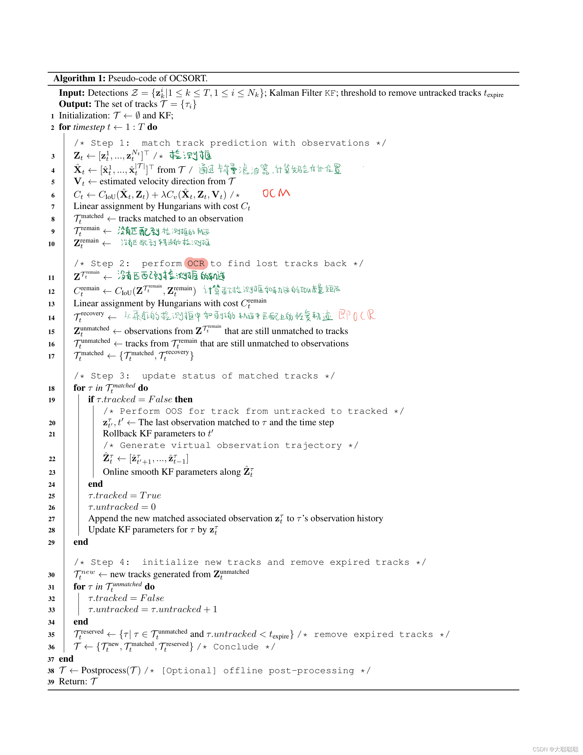

总结

在这里插入图片描述

匹配代码：
1.两阶段匹配，类似于bytetrack，两阶段都都是用的高分检测狂（置信度大于0.6的box）
2第一阶段匹配的轨迹：包括活跃的轨迹（没有丢失的轨迹）和不活跃的轨迹（30帧内未匹配的轨迹），两种轨迹都会通过卡尔曼滤波器得到预测框，然后进行匹配。
3第二阶段匹配的轨迹：为上一阶段未匹配的轨迹，但是不是卡尔曼滤波器预测的预测框，而是每个轨迹丢失时的位置（即轨迹丢失之前最后一帧的位置）。

 """
            First round of association
        """
        matched, unmatched_dets, unmatched_trks = associate(
            dets, trks, self.iou_threshold, velocities, k_observations, self.inertia)
        for m in matched:
            self.trackers[m[1]].update(dets[m[0], :])

        """
            Second round of associaton by OCR
        """

        

        if unmatched_dets.shape[0] > 0 and unmatched_trks.shape[0] > 0:
            left_dets = dets[unmatched_dets]
            left_trks = last_boxes[unmatched_trks]
            iou_left = self.asso_func(left_dets, left_trks)
            iou_left = np.array(iou_left)
            if iou_left.max() > self.iou_threshold:
                """
                    NOTE: by using a lower threshold, e.g., self.iou_threshold - 0.1, you may
                    get a higher performance especially on MOT17/MOT20 datasets. But we keep it
                    uniform here for simplicity
                """
                rematched_indices = linear_assignment(-iou_left)
                to_remove_det_indices = []
                to_remove_trk_indices = []
                for m in rematched_indices:
                    det_ind, trk_ind = unmatched_dets[m[0]], unmatched_trks[m[1]]
                    if iou_left[m[0], m[1]] < self.iou_threshold:
                        continue
                    self.trackers[trk_ind].update(dets[det_ind, :])
                    to_remove_det_indices.append(det_ind)
                    to_remove_trk_indices.append(trk_ind)
                unmatched_dets = np.setdiff1d(unmatched_dets, np.array(to_remove_det_indices))
                unmatched_trks = np.setdiff1d(unmatched_trks, np.array(to_remove_trk_indices))

Benchmark Performance

时间：2022.4.24
benchmark performance

大聪聪聪

关注

15
点赞
踩
73

收藏

觉得还不错? 一键收藏
5
评论
论文阅读：Observation-Centric SORT: Rethinking SORT for Robust Multi-Object Tracking——OC-SORT

文章提出了一种用于多目标跟踪的算法Obeservation-Centric SORT(OC-SORT),以解决多目标跟踪中模型对目标重叠、非线性运动的敏感和需要高帧率视频的问题。
复制链接

扫一扫