


第三讲 gradient_decent 源代码和 stochastic_gradient_decent 源代码。
B站 刘二大人 ,传送门PyTorch深度学习实践——梯度下降算法
参考错错莫课代表的PyTorch 深度学习实践 第3讲
笔记如下:

gradient_decent 源代码
import matplotlib.pyplot as plt

# set traindata
x_data = [1.0, 2.0, 3.0]
y_data = [2.0, 4.0, 6.0]

# initial weight
w = 1.0

# define the linear function y = w*x
def forward(x):
    return x*w

# define the cost function MSE
def cost(xs, ys):
    cost = 0
    for x,y in zip(xs,ys):
        y_pred = forward(x)
        cost += (y_pred-y)**2
    return cost / len(xs)

def gradient(xs,ys):
    grad = 0
    for x,y in zip(xs,ys):
        grad += 2*x*(x*w - y)
    return grad / len(xs)

epoch_list = []
cost_list = []
print('predict (before training)', 4, forward(4))
for epoch in range(100):
    cost_val = cost(x_data, y_data)
    grad_val = gradient(x_data, y_data)
    w -= 0.01*grad_val # 学习率为0.01
    print('epoch:', epoch, 'w=%.2f' %w, 'loss=%.2f' %cost_val)
    epoch_list.append(epoch)
    cost_list.append(cost_val)

print('predict (after training)', 4, forward(4))
plt.plot(epoch_list,cost_list)
plt.xlabel('epoch')
plt.ylabel('cost')
plt.show()
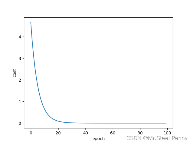
可视化效果:
部分输出结果:
predict (before training) 4 4.0
epoch: 0 w=1.09 loss=4.67
epoch: 1 w=1.18 loss=3.84
epoch: 2 w=1.25 loss=3.15
epoch: 3 w=1.32 loss=2.59
epoch: 4 w=1.39 loss=2.13
epoch: 5 w=1.44 loss=1.75
epoch: 6 w=1.50 loss=1.44.
epoch: 51 w=1.99 loss=0.00
epoch: 52 w=1.99 loss=0.00
epoch: 53 w=1.99 loss=0.00
epoch: 54 w=2.00 loss=0.00
epoch: 55 w=2.00 loss=0.00
epoch: 56 w=2.00 loss=0.00.
epoch: 97 w=2.00 loss=0.00
epoch: 98 w=2.00 loss=0.00
epoch: 99 w=2.00 loss=0.00
predict (after training) 4 7.999777758621207这里输出和视频里不太一样,本来是浮点数,我后来给取保留两位小数。
总体可以看出权重 w 收敛在2处。
随机梯度下降法在神经网络中被证明是有效的。
| 方法 | Gradient Descent | Stochastic Gradient Descent | Mini-Bach |
| 学习性能 | 低 | 高 | 适中 |
| 时间复杂度 | 低 | 高 | 适中 |
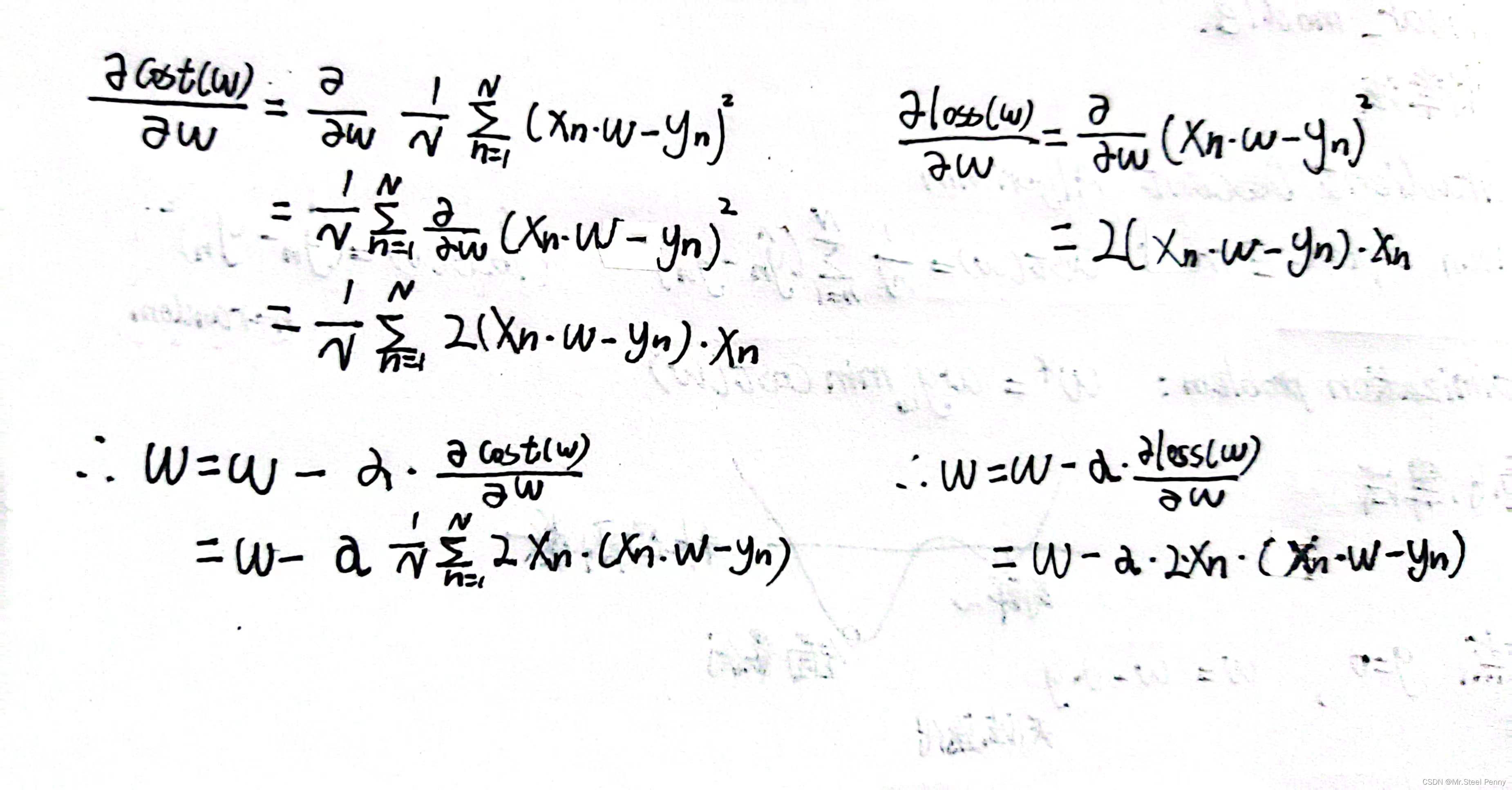
这两个算法的主要区别就是相比于梯度下降法这种将所有样本的损失求均值的方法,随机梯度下降法是随机选出一个样本的损失来进行计算,因此对应的gradient函数和w迭代需要改变,具体公式如下(手推):
stochastic_gradient_decent 源代码
import matplotlib.pyplot as plt

# prepare the training set
x_data = [1.0, 2.0, 3.0]
y_data = [2.0, 4.0, 6.0]

# initial guess of weight
w = 1.0


# define the model linear model y = w*x
def forward(x):
    return x * w


# define the cost function MSE
def loss(x, y):
    y_pred = forward(x)
    loss = (y_pred - y) ** 2
    return loss

# define the gradient function  gd
def gradient(x, y):
    return 2 * x * (x * w - y)

epoch_list = []
loss_list = []
print('predict (before training)', 4, forward(4))
for epoch in range(100):
    for x,y in zip(x_data, y_data):
        grad = gradient(x, y)
        w -= 0.01*grad  # update weight by every grad of sample of training set
        print("\tgrad:", x, y, grad)
        l = loss(x, y)
    print('epoch:', epoch, 'w=%.2f' %w, ' loss=%.2f' %l)
    epoch_list.append(epoch)
    loss_list.append(l)

print('predict (after training)', 4, forward(4))
plt.plot(epoch_list, loss_list)
plt.ylabel('loss')
plt.xlabel('epoch')
plt.show()
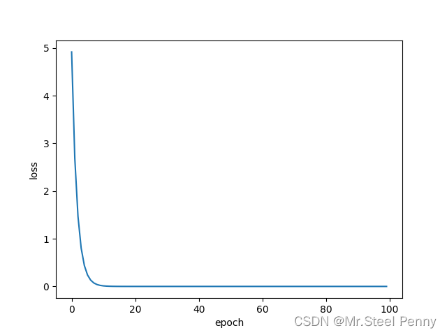
可视化效果:
部分输出结果:
predict (before training) 4 4.0
grad: 1.0 2.0 -2.0
grad: 2.0 4.0 -7.84
grad: 3.0 6.0 -16.2288
epoch: 0 w=1.26 loss=4.92
grad: 1.0 2.0 -1.478624
grad: 2.0 4.0 -5.796206079999999
grad: 3.0 6.0 -11.998146585599997
epoch: 1 w=1.45 loss=2.69
grad: 1.0 2.0 -1.093164466688
grad: 2.0 4.0 -4.285204709416961
grad: 3.0 6.0 -8.87037374849311
epoch: 2 w=1.60 loss=1.47
grad: 1.0 2.0 -0.8081896081960389
grad: 2.0 4.0 -3.1681032641284723
grad: 3.0 6.0 -6.557973756745939
epoch: 3 w=1.70 loss=0.80
grad: 1.0 2.0 -0.59750427561463
grad: 2.0 4.0 -2.3422167604093502
grad: 3.0 6.0 -4.848388694047353.
.
epoch: 16 w=1.99 loss=0.00
grad: 1.0 2.0 -0.011778821430517894
grad: 2.0 4.0 -0.046172980007630926
grad: 3.0 6.0 -0.09557806861579543
epoch: 17 w=2.00 loss=0.00
grad: 1.0 2.0 -0.008708224029438938
grad: 2.0 4.0 -0.03413623819540135
grad: 3.0 6.0 -0.07066201306448505.
.epoch: 98 w=2.00 loss=0.00
grad: 1.0 2.0 -2.0650148258027912e-13
grad: 2.0 4.0 -8.100187187665142e-13
grad: 3.0 6.0 -1.6786572132332367e-12
epoch: 99 w=2.00 loss=0.00
predict (after training) 4 7.9999999999996945


 1万+
1万+


 被折叠的 条评论
为什么被折叠?
被折叠的 条评论
为什么被折叠?
 到【灌水乐园】发言


