高斯随机数发生器（verilog实现）

zfmy_echo

已于 2024-03-25 16:56:14 修改

阅读量3.5k

点赞数 5

文章标签： verilog

于 2022-02-05 10:47:21 首次发布

本文链接：https://blog.csdn.net/weixin_52086903/article/details/122788471

版权

高斯随机数发生器（verilog实现）

文章目录

- 高斯随机数发生器（verilog实现）

一、理论部分

经查阅网络资料与文献，首先通过细胞自动机（cellular automata)获得均匀分布的随机变量，然后通过Box-Muller变换将均匀分布的随机变量变换为服从高斯分布的随机变量。

（一）细胞自动机

细胞自动机是一个细说起来十分复杂的概念，但是可以在我们的应用场景中可以得到简化。先放表达式
$s_i^{t+1}=f_i(s_{i-1}^{t},s_{i}^{t},s_{i+1}^{t})$
式中 $s_i^{t+1}$ 表示在t+1时刻第i个细胞的状态，它取决于t时刻第i-1个、第i个、第i+1个细胞的状态为自变量的某一种函数映射关系（ $f_i$ )。

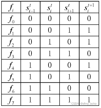
为了方便起见，将基本细胞自动机的邻域状态配置{ $s_i^{t-1}$ , $s_i^{t}$ , $s_i^{t+1}$ }的映射 { $f_7$ =(111), $f_6$ =(110),… $f_1$ =(001), $f_0$ =(000)} 的组合 $I_f$ = $\sum_{i=0}^{7}f_i2^i$ 称为基本细胞自动机的规则号。

例如{ $f_7f_6f_5f_4f_3f_2f_1f_0=10010110$ } 即 $150=2^1+2^2+2^4+2^7$ 对应的规则号是150。对于规则150，上述表达式可以写为
$s_i^{t+1}=s_{i-1}^{t}+s_{i}^{t}+s_{i+1}^{t}$
如下图

请添加图片描述

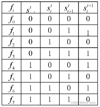
再如{ $f_7f_6f_5f_4f_3f_2f_1f_0=01011010$ } 即 $90=2^1+2^3+2^4+2^6$ 对应的规则号是90。对于规则90，上述表达式可以写为
$s_i^{t+1}=s_{i-1}^{t}+s_{i+1}^{t}$
如下图

请添加图片描述

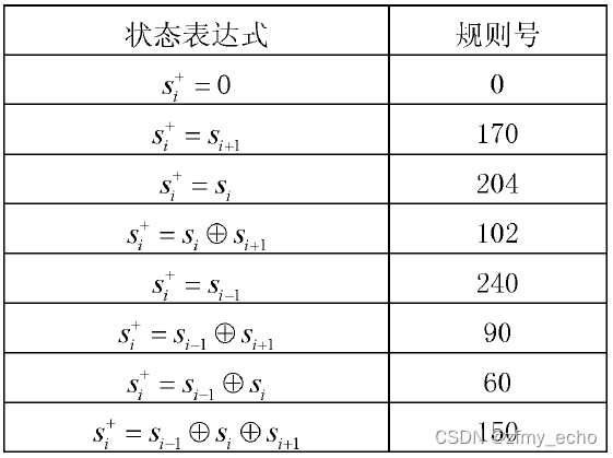
在这里贴上一些规则号与状态表达式的映射关系

请添加图片描述

（二）Box-Muller变换

Box-Muller变换是通过服从均匀分布 的随机变量，来构建服从高斯分布 的随机变量的一种方法。设 U1、U2为服从[0,1]上均匀分布的随机变量，若 X、**Y **满足
$X=cos(2\pi U_1 )\sqrt{-2lnU_2}\\ Y=sin(2\pi U_1 )\sqrt{-2lnU_2}$
则 X、Y 服从均值为0，方差为1的高斯分布。

以下是数学推导，若以实现功能为目的可自行跳过。

假定 X、Y 服从均值为0，方差为1的高斯分布，且相互独立。令p(X)和p(Y)分别为其密度函数，则
$\frac{1}{\sqrt{2\pi}}e^{-\frac{X^2}{2}}\\ p(Y)= \frac{1}{\sqrt{2\pi}}e^{-\frac{Y^2}{2}}$
由于X、Y相互独立，因此它们的联合概率密度满足
$p(X,Y)=\frac{1}{\sqrt{2\pi}}e^{-\frac{X^2+Y^2}{2}}$
将X、Y作坐标变换，使
$X=R\cos{\theta}\\ Y=R\sin{\theta}$
则
$\int_{-\infty}^{\infty}\int_{-\infty}^{\infty}\frac{1}{2\pi}e^{-\frac{X^2+Y^2}{2}}dXdY=\int_{-\infty}^{\infty}\int_{-\infty}^{\infty}\frac{1}{2\pi}e^{-\frac{R^2}{2}}Rd\theta dR=1$
由此可得R与θ的分布函数
$P_R(R\leq r)=\int_{0}^{2\pi}\int_0^{r}\frac{1}{2\pi}e^{-\frac{R^2}{2}}Rd\theta dR=1-e^{-\frac{r^2}{2}}\\ P_\theta(\theta\leq \phi)=\int_{0}^{\phi}\int_0^{\infty}\frac{1}{2\pi}e^{-\frac{R^2}{2}}Rd\theta dR=\frac{\phi}{2\pi}$
显然，θ服从[0,2π]上的均匀分布。令
$F_R(r)=1-e^{\frac{r^2}{2}}$
则其反函数
$R=F^{-1}_{R}=\sqrt{-2ln(1-z)}$
当z服从[0,1]上均匀分布时，R的分布函数为 $F_R(r)$ 。因此可以选择两个服从[0,1]上均匀分布的随机变量U1、U2，使得
$U_1 = \frac{\theta}{2\pi}, U_2 = 1-z$
即
$\theta = 2\pi U_1,R=\sqrt{-2lnU_2}$
将其带入
$X=R\cos{\theta}, Y=R\sin{\theta}$
得到最终表达式
$X=cos(2\pi U_1 )\sqrt{-2lnU_2}\\ Y=sin(2\pi U_1 )\sqrt{-2lnU_2}$

二、实践部分

（一）一维细胞自动机的实现

对于单个细胞

  always @(*)
  begin
    case({head,tail})
      2'b10:self_next = ctrl ? self^right:right;
      2'b01:self_next = ctrl ? left^self : left;
      2'b00:self_next = ctrl ? left^self^right:left^right;
      default:self_next=ctrl ? left^self^right:left^right;
    endcase
  end

head,tail用于判断该细胞是否处于队头或队尾。对头则无左侧细胞，队尾则无右侧细胞。

self_next 是该细胞下一时刻的值。

self、left、right 为本细胞、左侧细胞、右侧细胞的当前值。

ctrl用于判断规则号，这里只用到了规则150和规则90，分别以1和0表示。

当ctrl==1时，self_next =left ^ self ^ right，即规则150。

当ctrl==0时，self_next =left ^ right，即规则90。

对于N位的一维细胞自动机，只需要将上述单个细胞例化N次，并给出细胞的初始值和不同位置的规则号。

例如，对于32位自动细胞机，可以给出

parameter INIT_VEC = 32'b0100_1000_0001_0010_0100_1000_0001_0010,//初始值
parameter RULE_VEC = 32'b0000_1100_0100_0111_0000_1100_0000_0110,//规则号ctrl

通过使用generate语句简化例化过程。

generate
 genvar i;
  for(i=0; i<N; i=i+1) begin
   if (i==0) begin
    SingleCell#(.init(INIT_VEC[i]),.head(1'b0),.tail(1'b0)) 
    inst_SingleCell(    
           .clk_i   (clk_i),  
           .ctrl    (RULE_VEC[i]),
           .left    (1'b0),
           .right   (uni_r[1]),
           .self    (uni_r[i]),
           .out     (uni_next[i])
       );
   end
   ......//省略部分内容减少篇幅
endgenerate

一般的语法流程不再赘述，只展示关键部分。

为了检验生成的数据是否为服从均匀分布的随机变量，我们在对本模块仿真时导出数据为txt文本，并在matlab上展示出来。

仿真代码

`timescale 1ns / 1ps
module tb_CellAutomata();
localparam  INIT_VEC = 32'b0100_1000_0001_0010_0100_1000_0001_0010;
localparam  RULE_VEC = 32'b0000_1100_0100_0111_0000_1100_0000_0110;
localparam  N = 32;
localparam period = 10;
reg clk_i = 0;
reg rst_n_i = 1;
wire [N-1:0] uni_out;
CellularAutomata 
#(
  .INIT_VEC(INIT_VEC ),
  .RULE_VEC(RULE_VEC ),
  .N (N )
)
CellularAutomata_dut (
  .clk_i (clk_i ),
  .rst_n_i (rst_n_i ),
  .uni_out  (uni_out )
);
initial begin
  begin
    #(period*2) rst_n_i = 1'b0;
    #(period*10) rst_n_i = 1'b1;
    #(period*201_000);
    $writememb("new_data.txt",mem);
    $finish;
  end
end
parameter M = 200_000;
reg [N-1:0] mem [M:1];
integer index = 1;
initial begin//采集数据
    begin
        #(period*100);
        forever begin
            #(period);
            mem[index] = uni_out;
            index = (index >= M) ? 1 : index + 1;
        end
    end
  end
always
  #(period/2)  clk_i = !clk_i ;
endmodule

matlab部分

clear all;
clc;
fid = fopen("D:\MatlabProject\MatlabData\new_data.txt");
data = textscan(fid,"%b");
fclose(fid);
data = cell2mat(data);
data = double(data)/double(max(data));
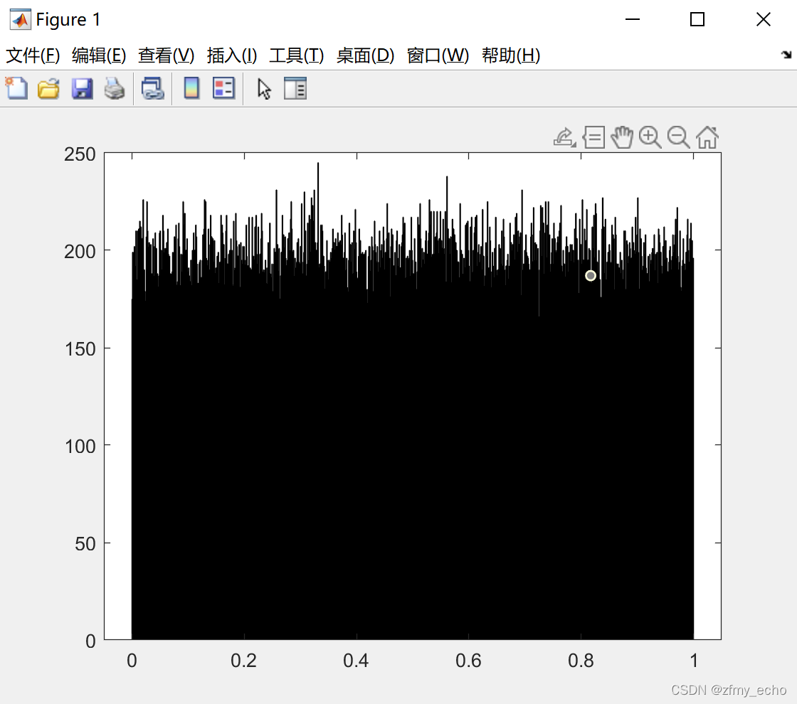
h = histogram(data,1024,"Binlimits",[0,1]);

可以看出虽然有些参差，但大致符合[0,1]上的服从均匀分布的随机变量。

请添加图片描述

（二）Box-Muller变换的实现

$X=cos(2\pi U_1 )\sqrt{-2lnU_2}\\ Y=sin(2\pi U_1 )\sqrt{-2lnU_2}$

本次选择了简易的方法近似实现函数。大致思路是，首先用matlab生成 $s in x$ 、 $cos x$ 、 $\sqrt{-2lnx}$ 函数自变量和因变量的映射，然后使IP核生成ROM并将其映射关系存放在ROM中，最后通过IP核生成乘法器将两部分相乘。

以 $s in$ 函数为例，给出matlab代码

clc;clear;                %储存单元地址线
depth=2^10;                 %存储单元;
widths=10;                    %数据宽度;
index = linspace(0,pi*2,depth);              
sin_value = sin(index); 
y1 = sin_value/max(sin_value);
sin_value = round(y1 * (depth/2 -1));  %扩大正弦幅度值    
plot(sin_value);
number = [0:depth];
fid=fopen('fsin.coe','w+');
fprintf(fid,'memory_initialization_radix=10;\n');
fprintf(fid,'memory_initialization_vector=\n');
for i = 1 : depth - 1  
    fprintf(fid, '%d,\n', sin_value(i));
end
fprintf(fid, '%d;', sin_value(depth));
fclose(fid);

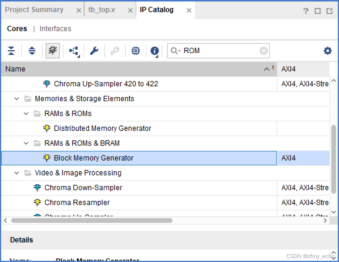
然后是IP核的使用。以Vivado2017.4为例。

第一步，点击IP Catalog，找到Block Memory Generator
请添加图片描述

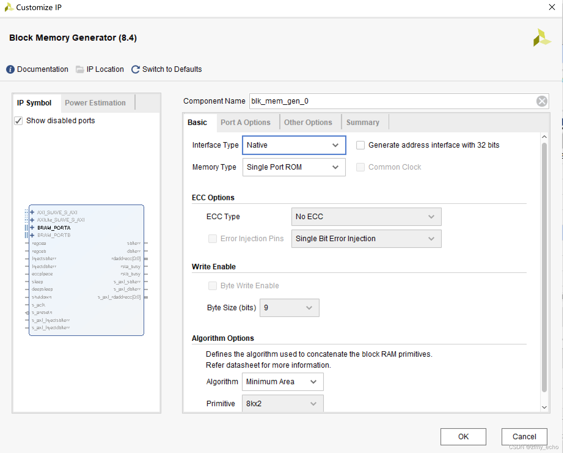
第二步，点击Block Memory Generator后进入Customize IP界面进行配置。

Basic界面中Memory Type使用 Single Port ROM即可。

请添加图片描述

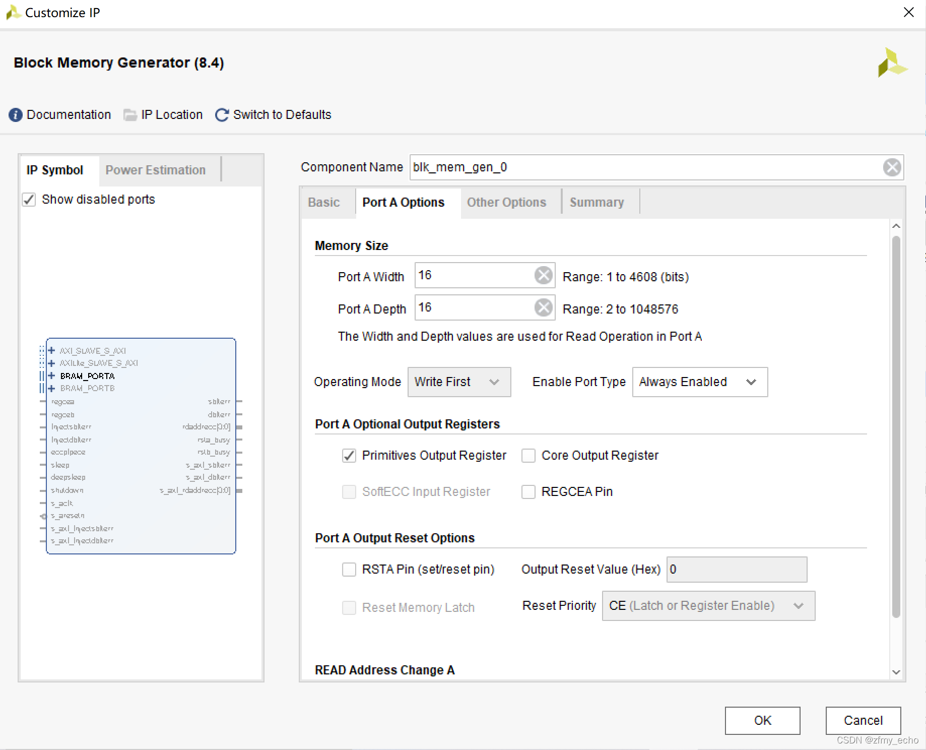
Port A Options中Port A Width决定了输出位宽，Port A Depth决定了输入地址的宽度。Enable Port Type 可以改成 Always Enabled，图个方便。

请添加图片描述

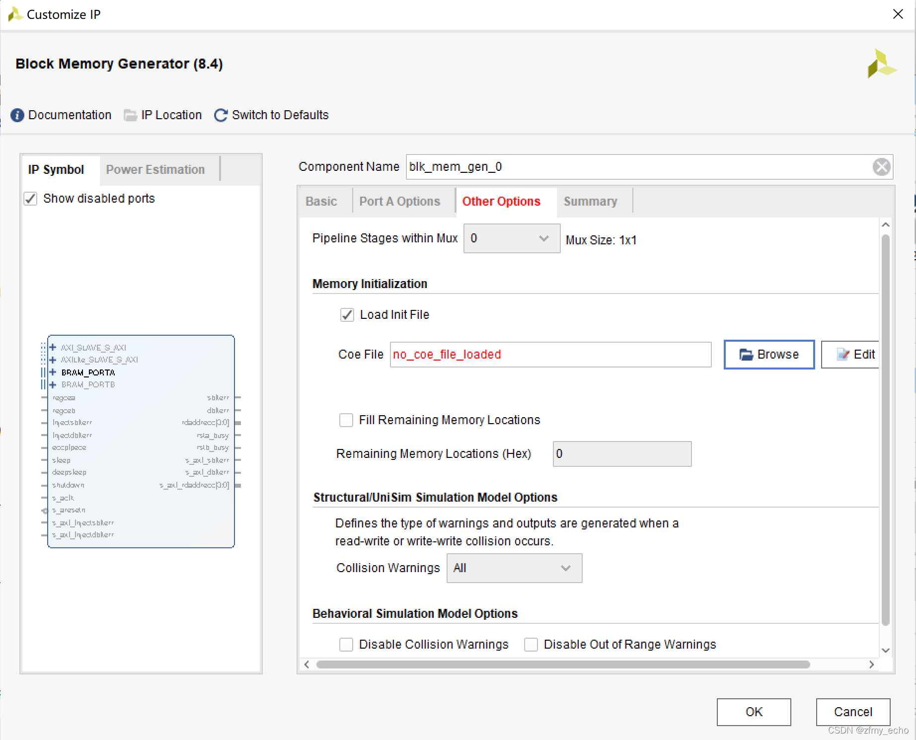
Other Options 界面中需要勾选 Load Init File 以将Matlab生成的.coe

文件导入。当文件格式、文件位置、文件中数据宽度不符合配置要求时都会标红。
请添加图片描述

Summary界面中可以看到一些相关信息，不再赘述。注意，当文件需要的IP核较多时，应当将IP核更改为条例清晰的命名以方便后续工作。生成完IP核后，使用时直接例化就ok了。乘法器IP核只需要找到 Multilplier核并配置即可，没有太大难度，不再演示。

按照有效果即可的原则（其实是电脑跑不动分析），我将原本计划的32位改为了20位输出。

module top_module(
    input clk_i,
    input reset,
    output wire [19:0]gaus1,
    output wire [19:0]gaus2
    );
    wire [31:0]uni_out;                  
    wire [9:0]addr1 = uni_out[9:0];
    wire [9:0]addr2 = uni_out[19:10];
    wire [9:0]value_sin;
    wire [9:0]value_cos;
    wire [9:0]value_y;
    CellularAutomata #(
      .INIT_VEC(32'b0100_1000_0001_0010_0100_1000_0001_0010 ),
      .RULE_VEC(32'b0000_1100_0100_0111_0000_1100_0000_0110 ),
      .N (32 ))
    CellularAutomata_dut (
      .clk_i (clk_i ),
      .reset (reset ),
      .uni_out  ( uni_out)
    );
    new 
    new_dut (
      .clk_i (clk_i ),
      .reset (reset ),
      .addr1 (addr1  ),
      .addr2 (addr2 ),
      .value_sin (value_sin ),
      .value_cos (value_cos ),
      .value_y  ( value_y)
    ); 
    Mult_Box_Muller inst1 (
      .CLK(clk_i),  // input wire CLK
      .A(value_sin),      // input wire [9 : 0] A
      .B(value_y),      // input wire [9 : 0] B
      .P(gaus1)      // output wire [19 : 0] P
    );
    Mult_Box_Muller inst2 (
      .CLK(clk_i),  // input wire CLK
      .A(value_cos),      // input wire [9 : 0] A
      .B(value_y),      // input wire [9 : 0] B
      .P(gaus2)      // output wire [19 : 0] P
    );
endmodule

（三）结果的仿真与检验

第一次仿真我得到了20位的输出，想要用Matlab读入数据时，发现我只会用Matlab读入16、32位这种整位的有符号数据，没有读入20位有符号数据的方法（没详细学过Matlab，别骂了别骂了），然后本着能用就用的原则，我把20位数据后加了12个0，凑到了32位。

仿真文件

`timescale 1ns / 1ps
module tb_top();
localparam period = 10;
reg clk_i = 0;
reg reset = 0;
wire [19:0] gaus1;
wire [19:0] gaus2;
reg [31:0]buffer1;
reg [31:0]buffer2;
always@(*)begin
  buffer1={gaus1,{12{1'b0}}};
  buffer2={gaus2,{12{1'b0}}};
end
parameter M = 65536;
reg [31:0] mem1 [M:1];
reg [31:0] mem2 [M:1];
integer index = 1;
top_module top_module_dut (
  .clk_i (clk_i ),
  .reset (reset ),
  .gaus1 (gaus1 ),
  .gaus2 (gaus2 )
);
integer k;
initial begin
for(k=1;k<(M+1);k=k+1) begin mem1[k] = 31'd0;mem2[k] = 31'd0; end
end
initial begin
  begin
    #(period*2)    reset = 1'b1;
    #(period*10)   reset = 1'b0;
    #(period*(M+1000));
    $writememb("gaus1.txt",mem1);
    $writememb("gaus2.txt",mem2);
    #(period*300);
    $finish;
  end
end
initial begin//采集数据
    begin
        #(period*12);
        forever begin
            #(period);
            mem1 [index] = buffer1;
            mem2 [index] = buffer2;
            index = (index >= M) ? 1 : index + 1;
        end
    end
end
always
  #(period/2)  clk_i = ! clk_i ;
endmodule

写的比较稍微有亿点点乱。将生成的数据用Matlab展示一下。

clear all;
clc;
fid = fopen("D:\MatlabProject\MatlabData\gaus1.txt");
data = textscan(fid,"%bs32");
fclose(fid);
data = cell2mat(data);
disp(data);
data = double(data)/pow2(32);
h = histogram(data, 1024,'BinLimits',[-1,1]);
%[h,p]=lillietest(data);
%normplot(data);

请添加图片描述

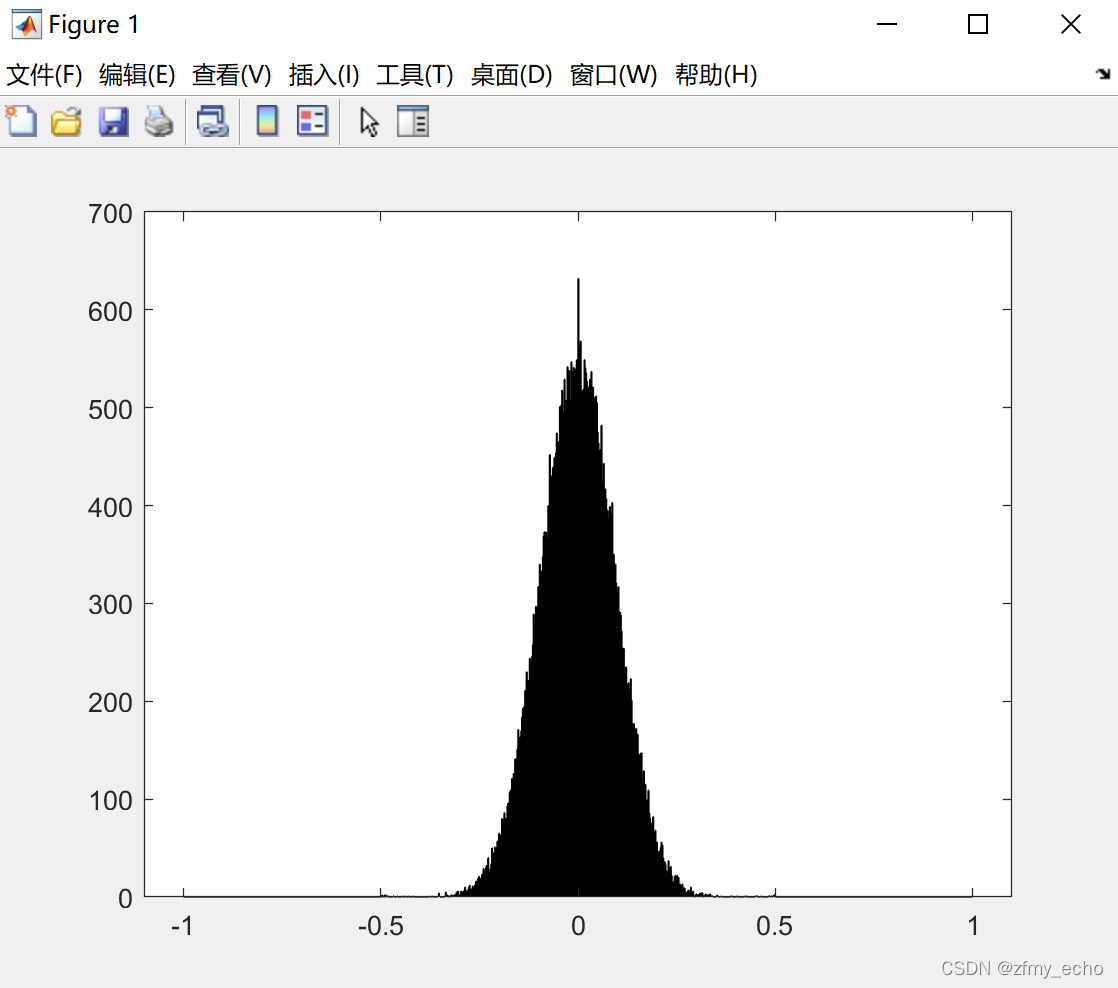
好像有点像高斯分布，为了验证，我查到了两种检测方法。没错，就是我注释了的那两句。

[h,p]=lillietest(data);

请添加图片描述

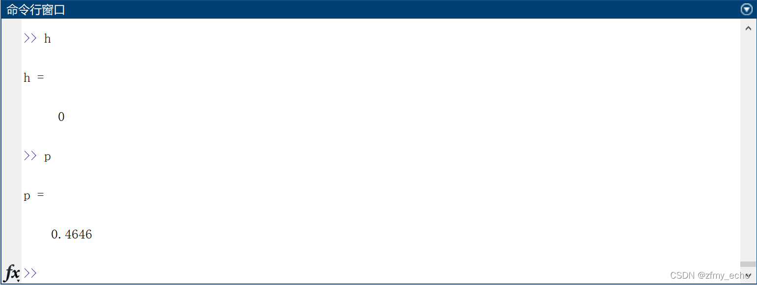
normplot(data);

请添加图片描述

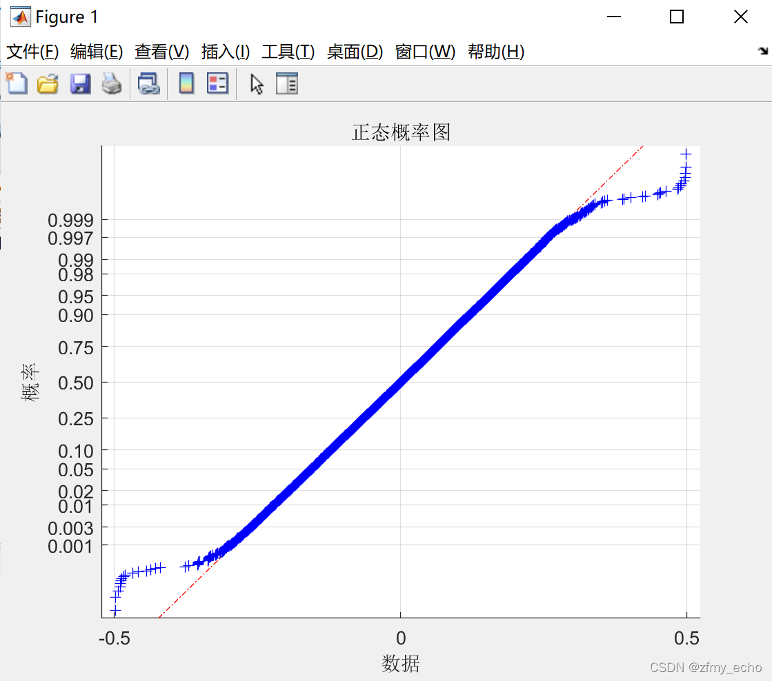
头尾较为稀疏且偏离较大，大概是因为原本数据只有20位数，强行加的12个0导致边缘稀疏。

三、一些感想

现在是2022年大年初四，立春，北京冬奥会开幕式。本来想写一下总结的，但是快到凌晨，所以不想了。新年快乐呀！

zfmy_echo

关注

5
点赞
踩
28

收藏

觉得还不错? 一键收藏
1
评论
高斯随机数发生器（verilog实现）

第一次仿真我得到了20位的输出，想要用Matlab读入数据时，发现我只会用Matlab读入16、32位这种整位的有符号数据，没有读入20位有符号数据的方法（没详细学过Matlab，别骂了别骂了），然后本着能用就用的原则，我把20位数据后加了12个0，凑到了32位。函数自变量和因变量的映射，然后使IP核生成ROM并将其映射关系存放在ROM中，最后通过IP核生成乘法器将两部分相乘。对于N位的一维细胞自动机，只需要将上述单个细胞例化N次，并给出细胞的初始值和不同位置的规则号。没错，就是我注释了的那两句。
复制链接

扫一扫