海量数据多变化点相关时间序列研究（Matlab代码实现）

💥💥💞💞欢迎小可爱们来到本博客❤️❤️💥💥

🏆博主优势：🌞🌞🌞博客内容尽量做到思维缜密，逻辑清晰，真心希望可以帮助到大家。

⛳️座右铭：行百里者，半于九十。

📋📋📋本文目录如下：🎁🎁🎁

目录

💥1 概述

📚2 运行结果

🎉3 参考文献

🌈4 Matlab代码实现

💥1 概述

当在研究识别随机过程中的结构变化时，会遇到两个挑战，一是以计算可处理的方式对具有依赖结构的时间序列进行分析。另一个挑战是，真实变化点的数量通常是未知的，需要合适的模型选择标准才能得出信息性的结论。首先解决第一个挑战，我们将数据生成过程建模为逐段自回归，它由几个段（时间纪元）组成，每个段都由自回归模型建模。我们提出了一种多窗口方法，该方法对于发现结构变化既有效又高效。所提出的方法是将分段自回归转换为渐近分段独立且相同分布的多元时间序列。解决第二个挑战，我们获得了（几乎肯定）选择分段独立多元时间序列的真实变化点数的理论保证。具体来说，在温和的假设下，我们表明类似贝叶斯信息准则（BIC）的标准给出了最佳变化点数量的强一致性选择，而类似赤池信息准则（AIC）的标准则不能。本文章说明了关于美国东部夏季温度的时间变化，以及海洋对气候影响的最主要因素，这也是环境科学家发现的。

📚2 运行结果

 

 

 

 部分代码如下！

% Harvard University 
% Created: December 2015
% Modified: May 2016

%% This file is about multiwindow detection algorithm for massive time series data
% it does not give an exact ordered clustering (since the ordered k means achives local maximum)
% synthetic data gives satisfying result 
% real data gives meaning result 
% NOTE: this clustering is for AR, and inside it uses ordered kmeans for IID data clustering 

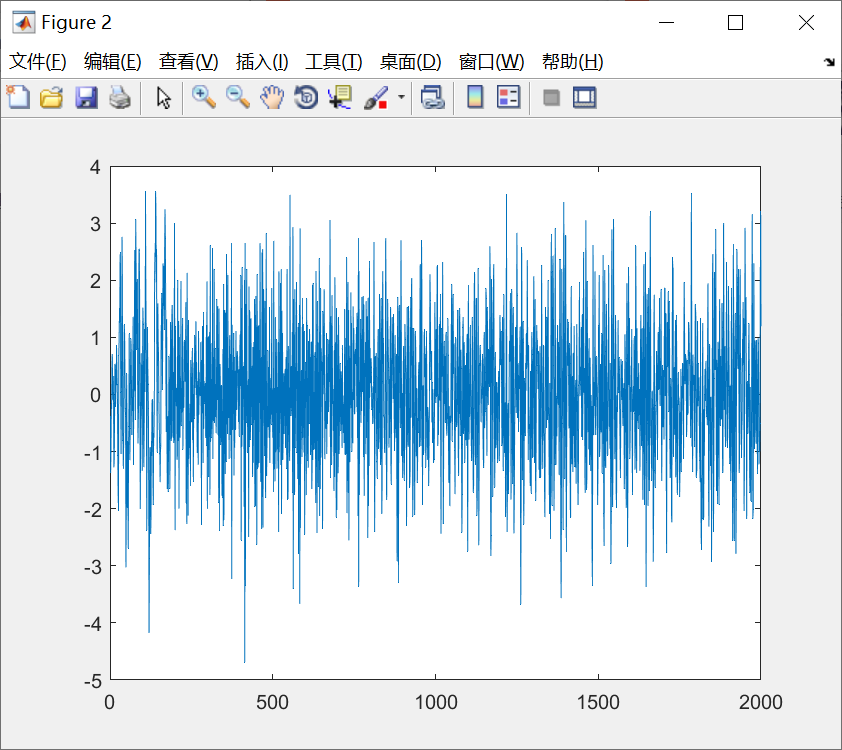
%% Synthetic data example: AR time series with one change point 
N = 2000;
N1 = floor(0.1*N);
N2 = floor(0.3*N);
L = 2;
a1 = [0.8 -0.3]; c1 = 0; %the first AR and constant
a2 = [-0.5 0.1]; c2 = 0; %the second AR and constant
a3 = [0.5 -0.5]; c3 = 0; %the third AR and constant
x = zeros(1,N);
x(1:L) = randn(1,L);
for n=L+1:N
    if n <= N1
        x(n) = x(n-1:-1:n-L) * a1' + c1 + randn;
    elseif n <= N1+N2
        x(n) = x(n-1:-1:n-L) * a2' + c2 + randn;
    else
        x(n) = x(n-1:-1:n-L) * a3' + c3 + randn;
    end
end
figure
plot(x)
windowSizes = [300 250 200 150 100 50]; 

%% Real data example 1: use MW method
% see the following reference for details
% Multiple Change Point Analysis: Fast Implementation And Strong Consistency, 
% Jie Ding, Yu Xiang, Lu Shen, and Vahid Tarokh, IEEE Transactions on Signal Processing, 2017.

whos -file ../data/NINO_monthly.mat
%load('../data/NINO_monthly.mat')
%x = NINO_monthly;

% set up window sizes 
windowSizes = [300 250 200 150 100 50]; 

%NOTE: x must be a row vector 
if (size(x,2) == 1)
    x = x';
end
 

%% %%%%%%%%%%%%%%%%%%%%%%%%%%%%%%%%%%%%%%%%%%% multi window detection %%%%%%%%%%%%%%%%%%%%%%%%%%%%%%%%%%%%%%%%%
L
N = length(x); 
nWindowType = length(windowSizes);

%search the suspicious region of size windowSize * range, it MAY OR MAY NOT depend on the window size
%range = 2;%floor(log(N));

%store the samples (estimated filters in each segment) for a particular window size
samples = cell(1,nWindowType); 

%the score for being a suspicious point 
score = zeros(1,N); 

tic
% %%%%%%%%%%%%%%%%%%%%%%%%%%%%%%%%%%%%%%%%%%% TURN windowed AR into iid Normal %%%%%%%%%%%%%%%%%%%%%%%%%%%%%%%%%%%%%%%%%%%
for n = 1:nWindowType 
    windowSize = windowSizes(n);
    nWindow = ceil(N/windowSize);
    samples{n} = zeros(nWindow, L+1);
    for k = 1:nWindow
        est = Estimate_1AR_Own_accelerate(x, 1+(k-1)*windowSize, min(k*windowSize,N), L);
        samples{n}(k,:) = est; %est(2:end)'; %SHOULD INCLUDE THE CONSTANT TERM
    end
    
    %===Global segmentation based on ordered k-means, note that K includes the default change point N 
    %choose the largest candidate number of segments 
    %THIS IS NECESSARY FOR REAL DATA
    %K = max( 2, ceil(log(nWindow)) ); 
    K=6;  
    penalty = (1:K)*1*sum(var(samples{n}))*2*log(log(nWindow)); %variance normalizing is helpful
    
    changePoints_candidates = cell(1,K);
    wgss_candidates = zeros(1,K);
    for k=1:K         
        %compute the best segmentation for each k
        [ changePoints_candidates{k}, wgss_candidates(k) ] = OrderKmeans(samples{n}, k, ceil(sqrt(nWindow))); 
    end
    [~, best_num_segments] = min( wgss_candidates + penalty );       
    changePoints = changePoints_candidates{best_num_segments}    
    
    %score the change points
    for k=1:length(changePoints)-1
        score( 1 + (changePoints(k)-1) * windowSize : min( (changePoints(k)+1) * windowSize, N ) ) = ...
            score( 1 + (changePoints(k)-1) * windowSize : min( (changePoints(k)+1) * windowSize, N ) ) + 1; 
    end
end
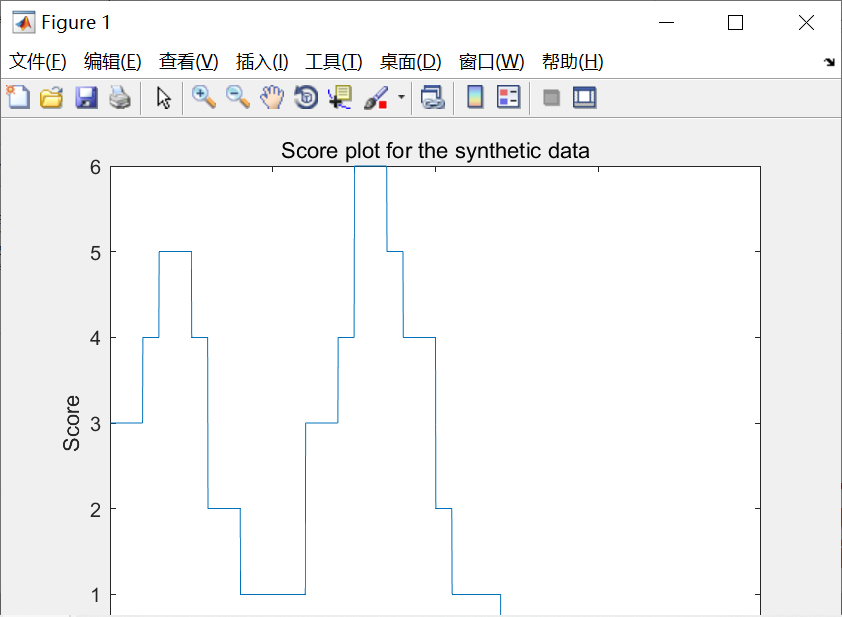
figure(1)
plot(score)
title('Score plot for the synthetic data')
xlabel('Time')
ylabel('Score')
%plot(1658+(1:N), score)
%plot(1854:1/12:2016-1/12, score)
toc
saveas(gcf, 'plot_synthetic.pdf') 
%saveas(gcf, '../results/plot_real1.pdf') 

%% Real data example 2: we can use exact search algorithm since the data size is small
whos -file ../data/EasternUS_yearly.mat
load('../data/EasternUS_yearly.mat')
x = EasternUS_yearly;

L = 0;

%[ changePoints1, wgss1 ] = exactSearch( yearlyData, 1, L )
%121  wgss1=53.6226

%[ changePoints2, wgss2 ] = exactSearch( yearlyData, 2, L )
%110   121 wgss2= 50.4418

%[ changePoints3, wgss3 ] = exactSearch( yearlyData, 3, L )
%35    45   121 wgss3=47.2979

%[ changePoints4, wgss4 ] = exactSearch( yearlyData, 4, L )
%35    50   110   121    wgss4 = 43.9876 

%[ changePoints5, wgss5 ] = exactSearch( yearlyData, 5, L )
%7    35    50   110   121   wgss5 = 41.3483

% [ changePoints6, wgss6 ] = exactSearch( yearlyData, 6, L)
%7    35    50   115   118   121   wgss6 = 39.0507

% [ changePoints6, wgss7 ] = exactSearch( yearlyData, 7, 7)
%7    35    50    85   115   118   121          wgss7 = 37.6790

% [ changePoints6, wgss6 ] = exactSearch( yearlyData, 8, L)
%7    35    50    57    61   115   118   121    wgss8 = 36.1572

wgss = [53.6226 50.4418  47.2979  43.9876  41.3483  39.0507 37.6790 36.1572];
[~,ind] = min( wgss + (0:7) * var(x) * 3 * log(log(121)) );
sprintf('num of change points is %d', ind-1)
 

🎉3 参考文献

部分理论来源于网络，如有侵权请联系删除。

[1]Jie Ding, Yu Xiang, Lu Shen, Vahid Tarokh (2017) Multiple Change Point Analysis for Massive Dependent Data

[2]梁建海,方英武,宋新海,苗壮.基于极值分段特征标识的时间序列分类方法[J].控制工程,2022,29(08):1528-1536.DOI:10.14107/j.cnki.kzgc.20200480.

[3]张森. 基于贝叶斯分层模型的物理数据融合分析[D].河北地质大学,2022.DOI:10.27752/d.cnki.gsjzj.2022.000782.

🌈4 Matlab代码实现