【全局灵敏性】【蒙特卡洛敏感性指数估计和多精度策略】基于方差的全局敏感性分析（Matlab代码实现）

 💥💥💞💞欢迎来到本博客❤️❤️💥💥

🏆博主优势：🌞🌞🌞博客内容尽量做到思维缜密，逻辑清晰，为了方便读者。

⛳️座右铭：行百里者，半于九十。

📋📋📋本文目录如下：🎁🎁🎁

目录

💥1 概述

📚2 运行结果

🎉3 参考文献

🌈4 Matlab代码、数据、文章

---

💥1 概述

当模型具有不确定的输入时，模型的输出也是不确定的。基于方差的全局敏感性分析通过将总方差分解为由每个不确定的输入和输入之间的相互作用导致的方差的百分比，来量化每个不确定输入对输出的相对影响。例如，Ishigami函数具有3个随机输入Z1、Z2和Z3，它们分布在区间[-𝜋,𝜋]上：

因此，Ishigami函数的方差可以分解为由单独的输入1、单独的输入2、单独的输入3以及输入1和2、输入1和3、输入2和3之间的相互作用，或者由所有三个输入之间的相互作用所引起的方差分量。这种分解被称为方差分析（ANOVA）分解，相当于将方差“馅饼”分解成不同的片段。对于上述的Ishigami函数（其中a=5，b=0.1），有40%的方差归因于Z1单独，29%的方差归因于Z2单独，31%的方差归因于Z1和Z3之间的相互作用。因此，方差“饼图”如下所示：

饼图，40%标记为Z1，29%标记为Z2，31%标记为Z1和Z3

全局敏感性指数量化了方差分解中每个输入的贡献。对于给定的输入，有两种不同的全局敏感性指数：

主效应敏感性指数，表示可以归因于该输入独自的方差百分比，即不考虑与其他输入之间的相互作用导致的影响，
总效应敏感性指数，表示受该输入影响的总方差百分比，包括仅由该输入产生的效应以及由该输入和其他输入产生的效应。
一般来说，所有输入的主效应敏感性指数之和为1或小于1，而所有输入的总效应敏感性指数之和为1或大于1。例如，在上述的Ishigami函数示例中，Z1、Z2和Z3的主效应敏感性指数分别为0.40、0.29和0，而总效应敏感性指数分别为0.71、0.29和0.31。

蒙特卡洛敏感性指数估计和多精度策略
主要效应和总效应敏感性指数可以使用蒙特卡洛估计进行估计。对于d个输入来估计主要和总效应敏感性指数，每个蒙特卡洛样本需要(d+2)个函数评估，因此当模型昂贵且d较大时，蒙特卡洛估计可能非常昂贵。我们提出多精度估计器，它结合了使用昂贵模型计算的少量高精度样本和使用更便宜的代理模型计算的许多低精度样本，以在固定的计算预算下提供比仅使用高精度模型更低方差的估计，同时保持高精度估计的准确性。

📚2 运行结果

部分代码：

%% COMPUTE MULTIFIDELITY GLOBAL SENSITIVITY ANALYSIS REPLICATES
n_reps = 100;    % number of replicates 
avg   = zeros(n_reps,2);    vr    = zeros(n_reps,2);
mc_sm = zeros(n_reps,d);    mc_st = zeros(n_reps,d);
mf_sm = zeros(n_reps,d);    mf_st = zeros(n_reps,d);

method = 'Gamboa';

for n = 1:n_reps
    
    % call mfsobol.m with just the high-fidelity model to get Monte
    % Carlo estimate
    [sm,st,mu,sigsq] = mfsobol(fcns(1),d,w(1),stats,budget,vec(1),method);
    avg(n,1) = mu; 
    vr(n,1) = sigsq;
    mc_sm(n,:) = sm;
    mc_st(n,:) = st;
    
    % call mfsobol.m with full array of functions to get multifidelity
    % estimates
    [sm,st,mu,sigsq] = mfsobol(fcns,d,w,stats,budget,vec,method);
    avg(n,2) = mu; 
    vr(n,2) = sigsq;
    mf_sm(n,:) = sm;
    mf_st(n,:) = st;
end

%% PLOT ESTIMATOR SPREAD
warning('off','MATLAB:legend:IgnoringExtraEntries')
blue = [0       0.4470 0.7410];
red  = [0.8500  0.3250 0.0908];

% plot main effect sensitivity indices
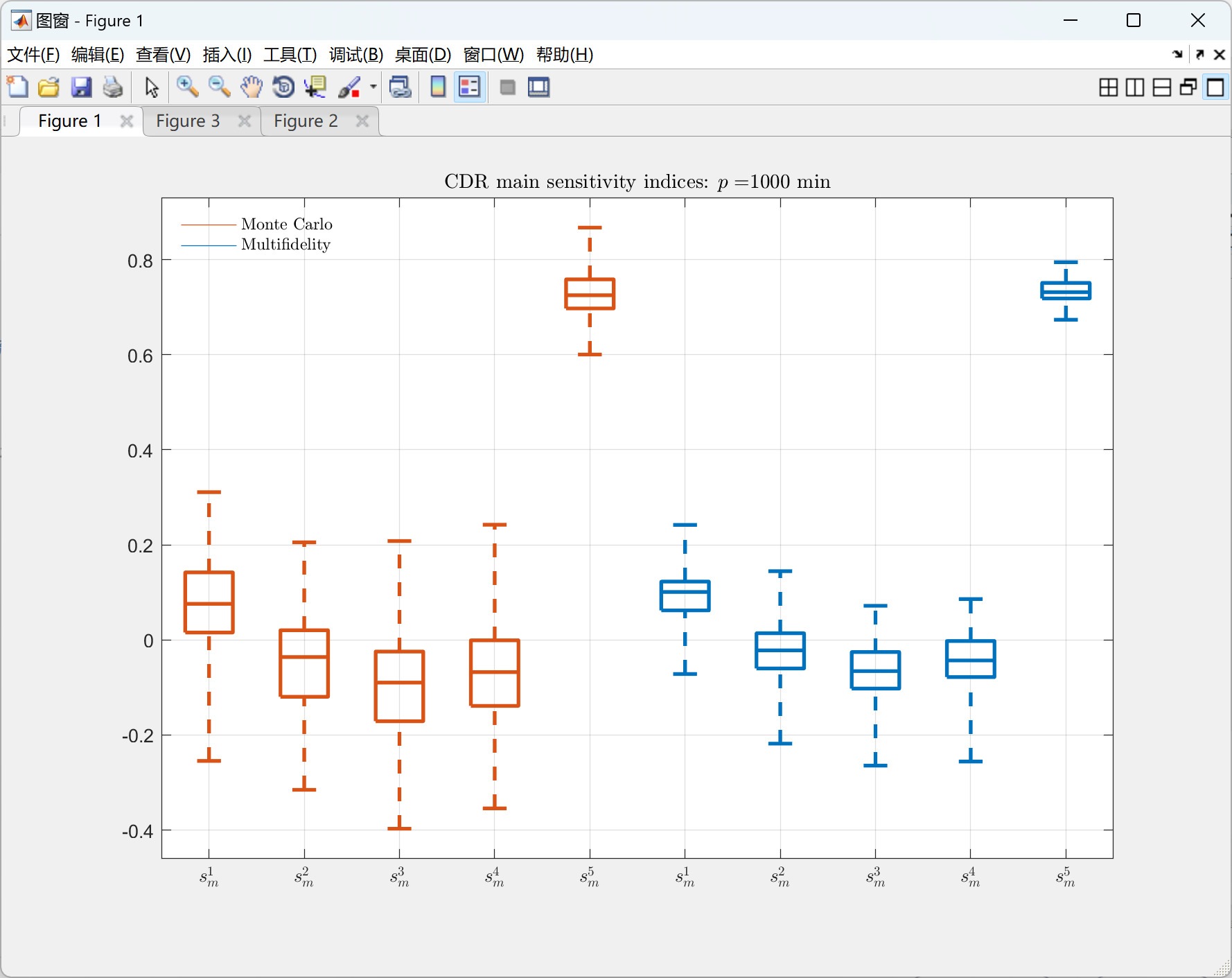
figure(1); clf
h = boxplot([mc_sm(:,1), mf_sm(:,1), mc_sm(:,2), mf_sm(:,2), mc_sm(:,3), mf_sm(:,3)],...
    'Colors',[blue; red; blue; red; blue; red],'Whisker',10,...
    'labels',{'MC $s_m^1$','MF $s_m^1$','MC $s_m^2$','MF $s_m^2$','MC $s_m^3$','MF $s_m^3$'});
set(h,{'linew'},{2}); grid on
legend(flipud(findall(gca,'Tag','Box')), {'High-fidelity estimate','Multifidelity estimate'},...
    'Location','SouthWest','interpreter','latex'); legend boxoff
bp = gca;   bp.XAxis.TickLabelInterpreter = 'latex';
title([method,' main sensitivity estimates for Ishigami function'],'interpreter','latex')

if strcmp(method,'Owen') || strcmp(method,'Saltelli')
    % plot total effect sensitivity indices
    figure(2); clf
    h = boxplot([mc_st(:,1), mf_st(:,1), mc_st(:,2), mf_st(:,2), mc_st(:,3), mf_st(:,3)],...
        'Colors',[blue; red; blue; red; blue; red],'Whisker',10,...
        'labels',{'MC $s_t^1$','MF $s_t^1$','MC $s_t^2$','MF $s_t^2$','MC $s_t^3$','MF $s_t^3$'});
    set(h,{'linew'},{2}); grid on
    hLegend = legend(flipud(findall(gca,'Tag','Box')), {'High-fidelity estimate','Multifidelity estimate'},...
        'Location','NorthEast','interpreter','latex'); legend boxoff
    bp = gca;   bp.XAxis.TickLabelInterpreter = 'latex';
    title([method,' total sensitivity estimates for Ishigami function'],'interpreter','latex')
end

% plot variance estimates
figure(3); clf
histogram(vr(:,1),12,'facecolor',blue); hold on
histogram(vr(:,2),12,'facecolor',red,'facealpha',1)
legend({'High-fidelity','Multifidelity'},'interpreter','latex'); legend boxoff
title('Variance estimates for Ishigami function','interpreter','latex')

🎉3 参考文献

文章中一些内容引自网络，会注明出处或引用为参考文献，难免有未尽之处，如有不妥，请随时联系删除。

 [1]王奇,陆林,李海阳,等.基于可控域的定点返回轨道全局敏感性分析[J].系统工程与电子技术, 2023, 45(11):3606-3615.DOI:10.12305/j.issn.1001-506X.2023.11.28.

[2]Gamboa, F., Gremaud, P., Klein, T., and Lagnoux, A. Global sensitivity analysis: A new generation of mighty estimators based on rank statistics, 2020.

[3]尹文进,张静远,饶喆,等.基于Sobol指数法作战能力全局敏感性分析方法[J].船电技术, 2015, 35(12):4.DOI:10.3969/j.issn.1003-4862.2015.12.005. 

[4]Gunzburger,Max,Peherstorfer,et al.OPTIMAL MODEL MANAGEMENT FOR MULTIFIDELITY MONTE CARLO ESTIMATION[J].Siam Journal on Scientific Computing, 2016.

🌈4 Matlab代码、数据、文章