【滤波跟踪】使用二维离散时间卡尔曼滤波器进行目标在二维平面上的跟踪，考虑了各种噪声强度（Matlab代码实现）

 💥💥💞💞欢迎来到本博客❤️❤️💥💥

🏆博主优势：🌞🌞🌞博客内容尽量做到思维缜密，逻辑清晰，为了方便读者。

⛳️座右铭：行百里者，半于九十。

📋📋📋本文目录如下：🎁🎁🎁

目录

💥1 概述

📚2 运行结果

🎉3 参考文献

🌈4 Matlab代码、数据

---

💥1 概述

二维离散时间卡尔曼滤波器是一种常用于目标跟踪的强大工具，它能够有效地处理系统模型和观测数据之间的不确定性和噪声。在目标跟踪中，通常会考虑目标在二维平面上的位置和速度。

首先，让我们定义系统的状态和观测模型：

1. **状态模型**：我们假设目标在二维平面上的位置和速度可以用一个状态向量来表示。假设状态向量为 \(x_k\)，其中 \(k\) 表示时间步，\(x_k = [p_x, p_y, v_x, v_y]^T\)，分别表示目标在 \(x\) 和 \(y\) 方向上的位置和速度。

   状态转移方程为：

   \[x_k = F_k \cdot x_{k-1} + w_k\]

   其中，\(F_k\) 是状态转移矩阵，通常为一个恒定矩阵，\(w_k\) 是系统过程噪声，假设为高斯分布，\(w_k \sim N(0, Q_k)\)，\(Q_k\) 是系统噪声协方差矩阵。

2. **观测模型**：我们假设可以通过某种传感器观测到目标的位置，但是观测值会受到噪声的影响。假设观测向量为 \(z_k\)，表示在时间步 \(k\) 观测到的目标位置。

   观测方程为：

   \[z_k = H_k \cdot x_k + v_k\]

   其中，\(H_k\) 是观测矩阵，通常是一个单位矩阵或者只提取位置信息的矩阵，\(v_k\) 是观测噪声，假设为高斯分布，\(v_k \sim N(0, R_k)\)，\(R_k\) 是观测噪声协方差矩阵。

接下来是卡尔曼滤波的步骤：

1. **初始化**：初始化状态向量 \(x_0\) 和状态协方差矩阵 \(P_0\)。

2. **预测**：根据状态转移方程预测下一个状态的状态向量 \(x_k\) 和状态协方差矩阵 \(P_k\)。

   \[x_k^- = F_k \cdot x_{k-1}\]
   \[P_k^- = F_k \cdot P_{k-1} \cdot F_k^T + Q_k\]

3. **更新**：根据观测值对预测值进行修正，得到最终的状态估计。

   \[K_k = P_k^- \cdot H_k^T \cdot (H_k \cdot P_k^- \cdot H_k^T + R_k)^{-1}\]
   \[x_k = x_k^- + K_k \cdot (z_k - H_k \cdot x_k^-)\]
   \[P_k = (I - K_k \cdot H_k) \cdot P_k^-\]

其中，\(K_k\) 是卡尔曼增益，\(I\) 是单位矩阵。

在实际应用中，系统参数如状态转移矩阵 \(F_k\)、系统噪声协方差矩阵 \(Q_k\)、观测矩阵 \(H_k\) 和观测噪声协方差矩阵 \(R_k\) 都需要根据具体问题进行调整和估计。通常情况下，这些参数可以通过系统建模、实验测试或者经验调整来确定。

📚2 运行结果

部分代码：

%% Kalman Filter params
R = [noise_x 0; 0 noise_y]; %coviarance of the noise
Q = [t^4/4 0 t^3/2 0; 0 t^4/4 0 t^3/2; t^3/2 0 t^2 0; 0 t^3/2 0 t^2].*noise^2; % covariance of the observation noise
P = Q; % estimate of initial state
F = [1 0 t 0; 0 1 0 t; 0 0 1 0; 0 0 0 1];  %state transition model
B = [1 0 0 0; 0 1 0 0];  %observation model
C = [(t^2/2); (t^2/2); t; t];  %control-input model
ksi_sta = []; % green node state
v = []; % green node velocity
y = []; % the measurements of the node state
ksi_sta_eta = []; %  initial state estimate
v_eta = []; % initial velocity estimate
P_eta = P;
pre_state = [];
pre_var = [];

%do the kalman filter and plot the origianl node and estimation node
for s = frame:length(img_file)
    img_tmp = double(imread(img_file(s).name));
    img = img_tmp(:,:,1);  % load the image
    y(:,s) = [ CM_idx(s,1); CM_idx(s,2)]; % load the given moving node
    
    ksi_eta = F * ksi_eta + C * u;
    pre_state = [pre_state; ksi_eta(1)] ;
    P = F * P * F' + Q; %Time Update
    pre_var = [pre_var; P] ;
    K = P*B'*inv(B*P*B'+R); %the Kalman Gain
    % Measurement Update
    if ~isnan(y(:,s))
        ksi_eta = ksi_eta + K * (y(:,s) - B * ksi_eta); %using the innovations signal
    end
   
    P =  (eye(4)-K*B)*P; % updated estimate covariance
    
    ksi_sta_eta = [ksi_sta_eta; ksi_eta(1:2)];
    v_eta = [v_eta; ksi_eta(3:4)];
    
    x_estimation(s)=ksi_eta(2); %estimation in horizontal position
    y_estimation(s)=ksi_eta(1); %estimation in vertical position
   
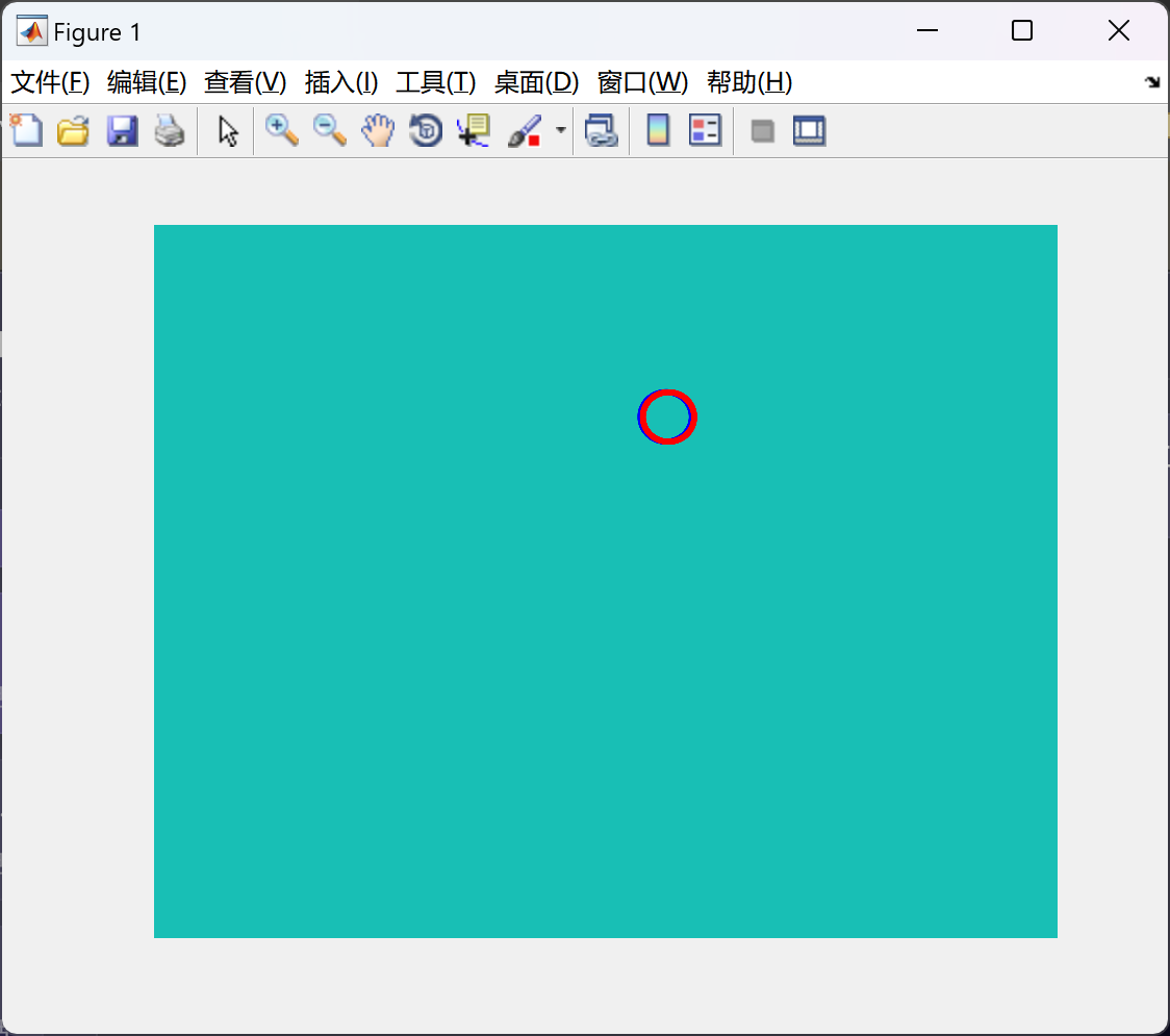
    r = 10;
    j=0:.01:2*pi; %parameters of nodes
    imagesc(img);
    axis off
    hold on;
    plot(r*sin(j)+y(2,s),r*cos(j)+y(1,s),'.b'); % the actual moving mode
    plot(r*sin(j)+ksi_eta(2),r*cos(j)+ksi_eta(1),'.r'); % the kalman filtered tracking node
    hold off
    pause(0.05) %speed of loading frame
end
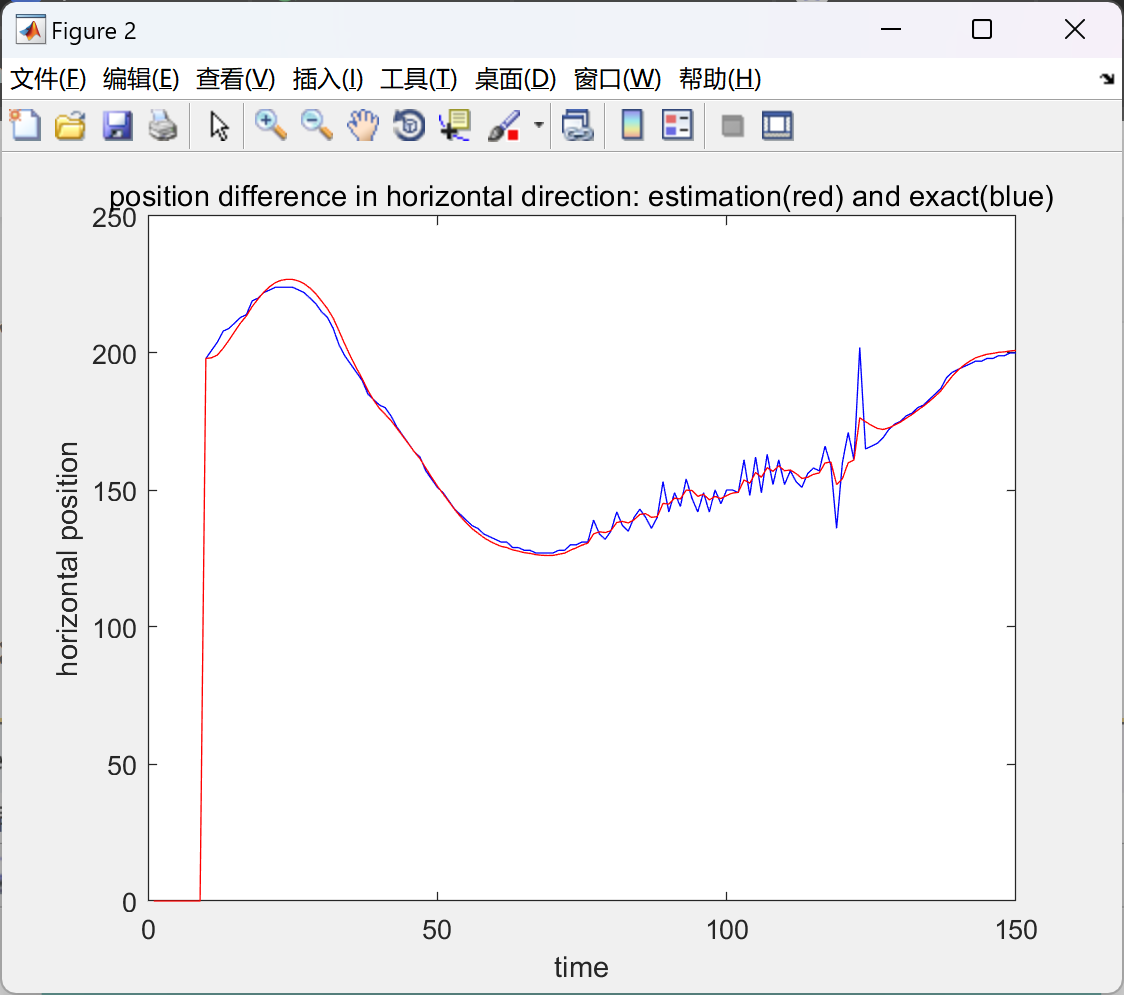
%show the position difference in horizontal direction between actual and estimation positions
l1=length(y(2,:)); n=1:l1;
figure;
plot(n,y(2,:),'b',n,x_estimation,'r');
xlabel('time'); ylabel('horizontal position');
title('position difference in horizontal direction: estimation(red) and exact(blue)');

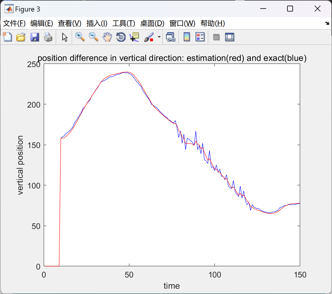
%show the position difference in vertical direction between actual and estimation positions
figure;
plot(n,y(1,:),'b',n,y_estimation,'r');
xlabel('time'); ylabel('vertical position');
title('position difference in vertical direction: estimation(red) and exact(blue)');

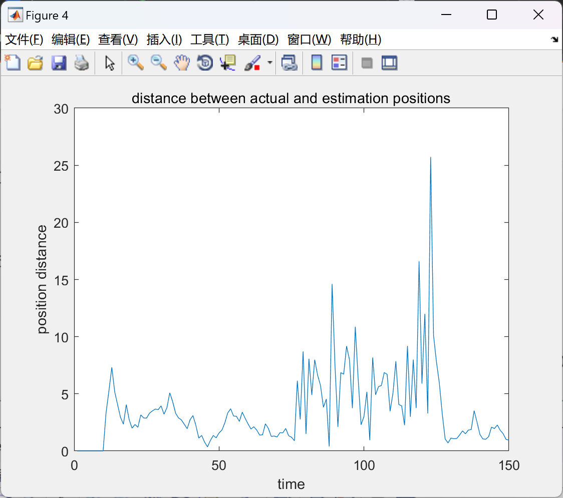
%show the distance between actual and estimation positions or error
x_d=y(2,:)-x_estimation;
y_d=y(1,:)-y_estimation;
xy_d=x_d.^(2)+y_d.^(2);
xy_d=xy_d.^(1/2);
figure;
plot(n,xy_d);
xlabel('time'); ylabel('position distance');
title('distance between actual and estimation positions');

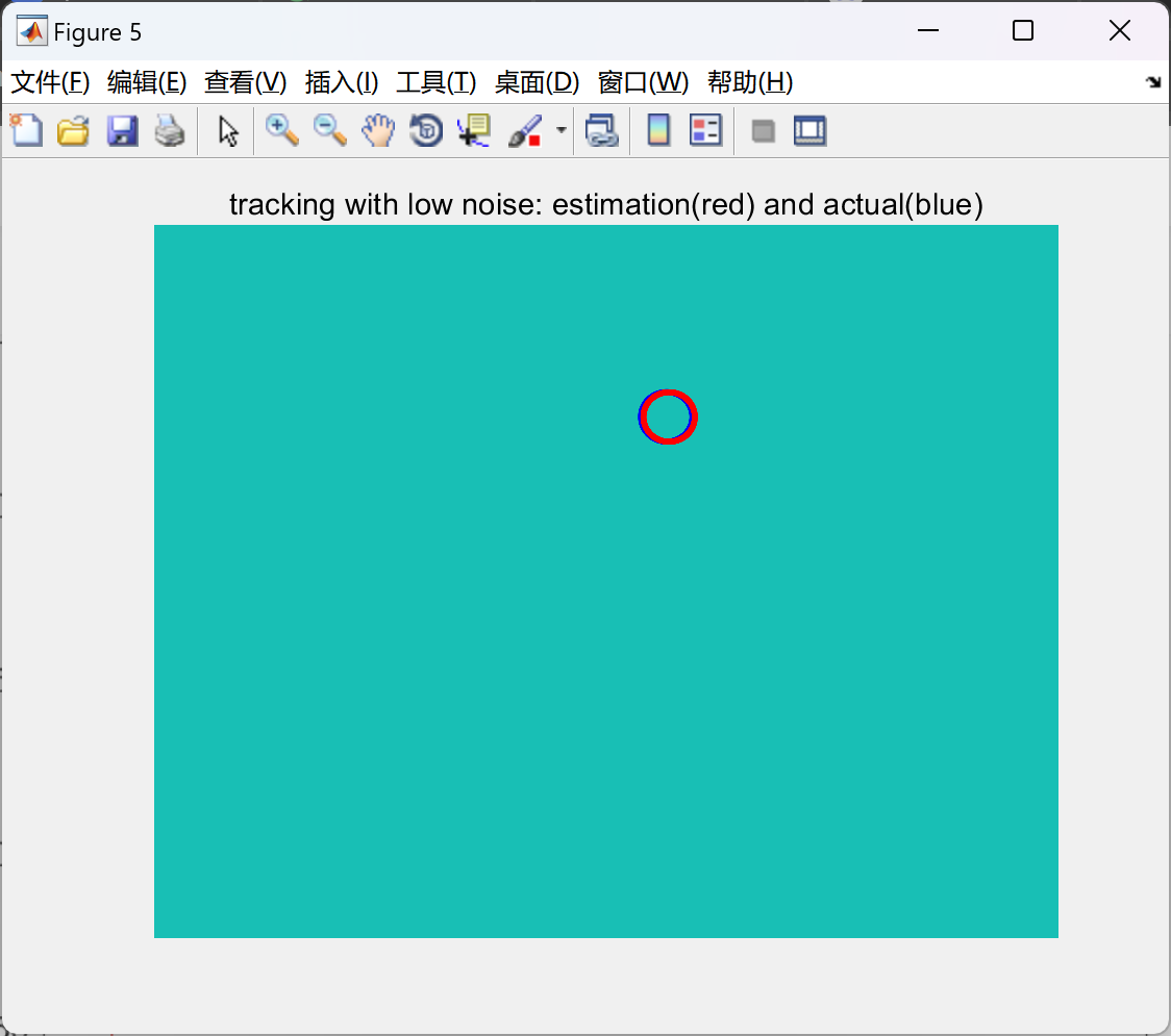
%show tracking with low noise
n_very_noisy=150;
img_tmp = double(imread(img_file(n_very_noisy).name));
img = img_tmp(:,:,1);  % load the image
figure;
imagesc(img);
axis off
hold on;
plot(r*sin(j)+y(2,n_very_noisy),r*cos(j)+y(1,n_very_noisy),'.b'); % the actual moving mode
plot(r*sin(j)+x_estimation(n_very_noisy),r*cos(j)+y_estimation(n_very_noisy),'.r'); % the kalman filtered tracking node
title('tracking with low noise: estimation(red) and actual(blue)');
hold off

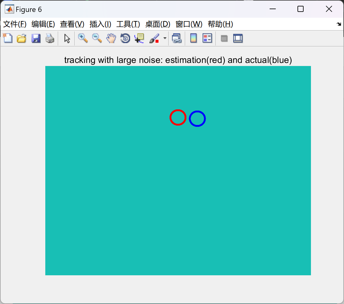
%show the mild noise tracking
%n_very_noisy=84;
%img_tmp = double(imread(img_file(n_very_noisy).name));
%img = img_tmp(:,:,1);  % load the image
%figure;
%imagesc(img);
%axis off
%hold on;
%plot(r*sin(j)+y(2,n_very_noisy),r*cos(j)+y(1,n_very_noisy),'.b'); % the actual moving mode
%plot(r*sin(j)+x_estimation(n_very_noisy),r*cos(j)+y_estimation(n_very_noisy),'.r'); % the kalman filtered tracking node
%title('tracking with mild noise: estimation(red) and actual(blue)');
%hold off

🎉3 参考文献

文章中一些内容引自网络，会注明出处或引用为参考文献，难免有未尽之处，如有不妥，请随时联系删除。

[1]崔璟琳.基于模糊卡尔曼滤波器的机动目标跟踪算法[J].科技资讯, 2008(9):2.DOI:CNKI:SUN:ZXLJ.0.2008-09-007.

[2]冯宜伟,李吉功,郭戈,等.基于Kalman滤波器的二维运动目标跟踪[J].石油化工高等学校学报, 2007, 20(3):4.DOI:10.3969/j.issn.1006-396X.2007.03.003.

[3]赵明冬,王继红.卡尔曼滤波算法在船用雷达运动目标跟踪滤波器中的应用[J].舰船科学技术, 2016(2X):3.DOI:CNKI:SUN:JCKX.0.2016-04-036.

🌈4 Matlab代码、数据