图机器学习基础知识——CS224W（02-tradition-ml）

CS224W: Machine Learning with Graphs

Stanford / Winter 2021

02-tradition-ml

Design features for nodes/links/graphs

Use hand-designed features

For simplicity, we focus on undirected graphs

• Traditional ML Pipeline

  • Hand-crafted feature + ML model

Node-level Tasks and Features

Goal: Characterize the structure and position of a node in the network

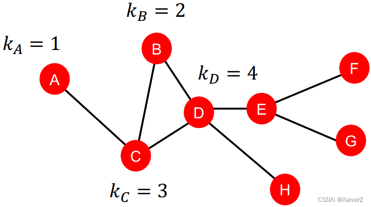
Node Degree

度

Importance-based features

Structure-based features

• $k_v$: the degree of node $v$

• 每个节点的特征为该节点的度

  

• Limitation

  • Treat all neighboring nodes equally, without capturing their importance

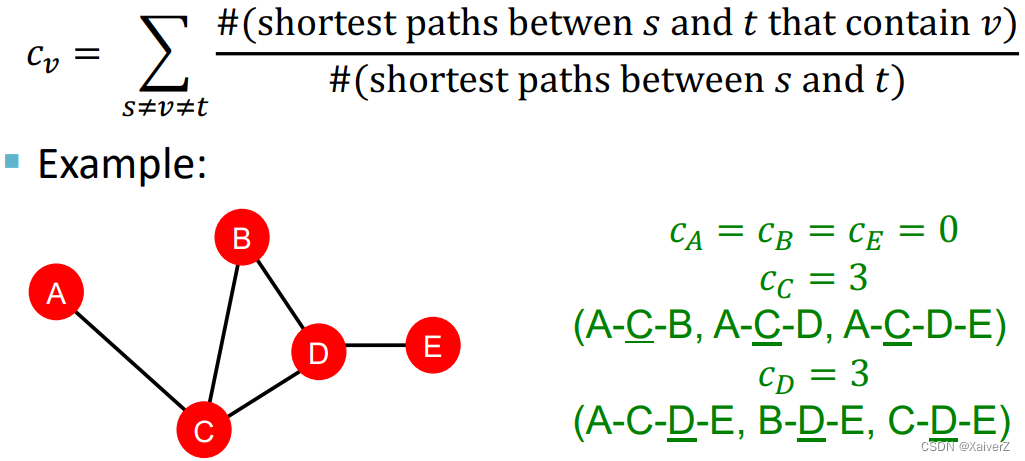
Node Centrality

中心性

Importance-based features

• $c_v$: node centrality of node $v$

• Node centrality $c_v$ takes the node importance in a graph into account

Engienvector Centrality

Engienvector Centrality

• Key Idea: A node $v$ is important if surrounded by important neighboring nodes $u\in N(v)$

• We model the centrality of node $v$ as the sum of the centrality of neighboring nodes

  $$c_v=\frac{1}{\lambda }\sum _{u\in N(v)}{c}_u$$
  $\lambda$ is some positive constant

• 上式是以递归形式（Recursive Manner）定义的，将其重写为矩阵形式（Matrix Form）

  $$\lambda \mathbf{c}=\mathbf{A}\mathbf{c}$$
  $\mathbf{A}$: (Sub-) Adjacency matrix, ${\mathbf{A}}_{uv}=1$ if $u\in N(v)$; $\mathbf{c}$: Centrality vector of node $v$

  • 从矩阵形式可以看出，节点中心性向量其实就是子邻接矩阵的特征向量

  • The largest eigenvalue ${\lambda }_{max}$ is always positive and unique (by Perron-Frobenius Theorem)

  • The leading eigenvector ${\mathbf{c}}_{max}$, which corresponds to the largest eigenvalue ${\lambda }_{max}$, is used for centrality

Betweenness Centrality

Betweenness Centrality

• Key Idea: A node is important if it lies on many shortest paths between other nodes (something like transit hub)

  

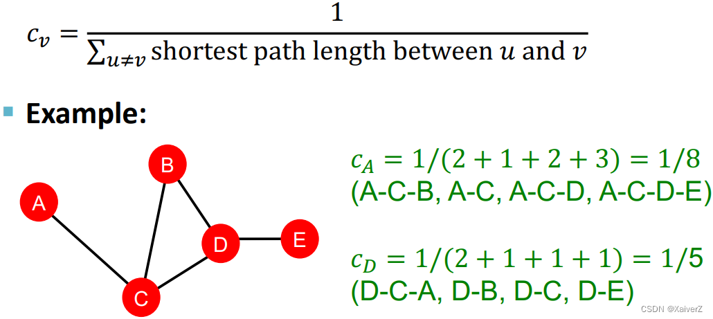
Closeness Centrality

Closeness Centrality

• Key Idea: A node is important if it has small shortest path lengths to all other nodes (其余节点到该节点的最短路径长度之和越小，该节点越重要，因为这样的节点一般处于中心位置，到其余节点的距离最短)

  

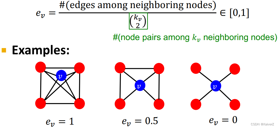
Clustering Coefficient

聚类系数

Structure-based features

• Key Idea: Measures how connected $v$’s neighboring nodes are (衡量节点$v$的邻居节点的连接程度)

  

  • 除了与节点$v$的邻居关系，聚类系数计算过程与节点$v$本身没有直接的关系

    • 以图1为例，$e_v$的分子为邻居节点之间的实际连边数，即为6（抹去$v$以及与其相连的边，剩下的即为邻居节点的边）；$e_v$的分母为组合数，从$v$的$k_v$个邻居节点中任选两点进行连边，计算最大连边总数

Graphlets

有根、连接的、非同构子图（Rooted connected non-isomorphic subgraphs）

• 以2-node graphlet为例，只有一种连接方式，且根节点的位置无论在哪个节点都是同构的，所以只有一种形式的有根连接非同构子图

• 以3-node graphlet为例，有两种连接方式，在第一种连接方式$G_1$中，根节点在两端以及在中心这两种情况是非同构的，所以$G_1$其实有两种有根连接非同构子图；在第二种连接方式$G_2$中，根节点无论在哪个点都是同构的，所以$G_2$只有一种有根连接非同构子图。总的来说，3-node graphlet共有三种有根连接非同构子图

  

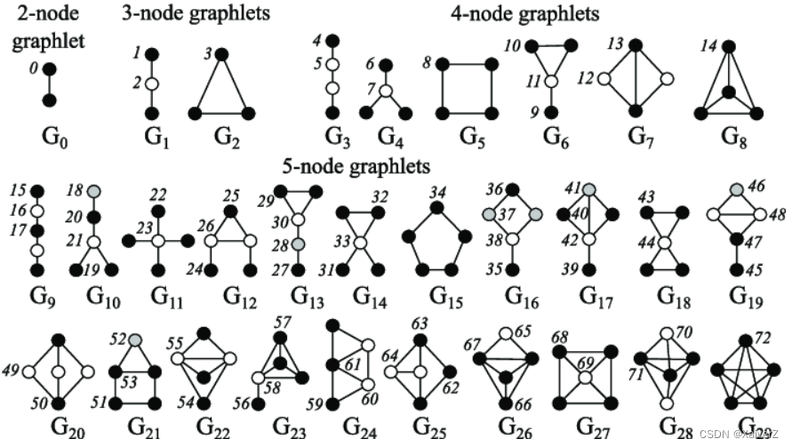
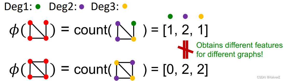
Graphlet Degree Vector (GDV)

Graphlet-base features for nodes, which counts #(graphlets) that a node touches

Structure-based features

• Key Idea: A count vector of graphlets rooted at a given node

  

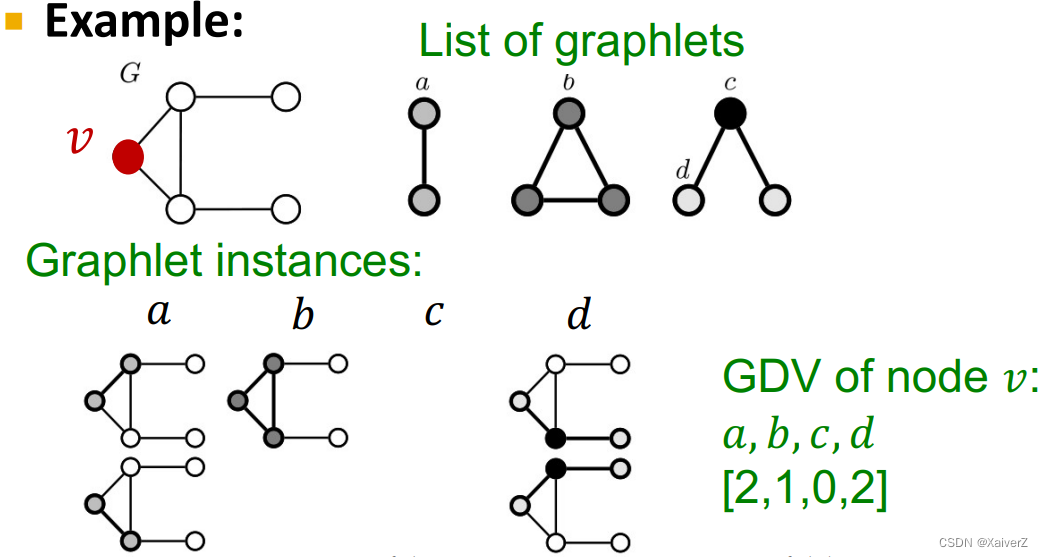
  • 如上图所示，只考虑2-3 nodes graphlets，共有四种有根连接非同构子图的形式，根节点分别为$a$、$b$、$c$、$d$

  • 在计算节点$v$的GDV时，以$v$为根节点分别去匹配四种graphlets的形式，并计数

  • Tips：根节点$c$的graphlet匹配数为0，因为原图以$v$为根节点的“三角形”有三条连边，而以$c$为根节点的graphlet只有两条连边（Graphlets的定义：有根、连接、非同构，缺一不可）

• 如果考虑2-5 nodes graphlets，那么

  • 会得到73种有根连接非同构子图，描述了节点周围邻居的拓扑结构

  • 捕捉到4跳以内距离（distance of 4 hops）的节点互连关系

• Graphlet degree vector (GDV) provides a measure of a node’s local network topology

Link-level Tasks and Features

Goal: To predict new links based on existing links

At test time, all node pairs (no existing links) are ranked, and top $K$ node pairs are predicted

Key: To design features for a pair of nodes

• Two formulations of the link prediction task

  • Links missing at random

    Remove a random set of links and then aim to predict them

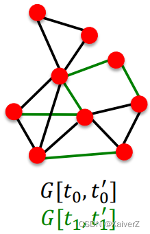
  • Links over time

    Assume that our network evolves over time (e.g. social network) and new links will be added in the future. Give $G[t_0,t_0^{\prime }]$ a graph on edges up to time $t_0^{\prime }$, output a ranked list $L$ of links (not in $G[t_0,t_0^{\prime }]$) that are predicted to appear in $G[t_1,t_1^{\prime }]$

    • Evaluation: Take top n elements of $L$ and count correct edges that actually appear in test period $[t_1,t_1^{\prime }]$

    

• Link Prediction via Proximity

  • For each pair of nodes $(x,y)$ compute score $c(x,y)$

    • As an example, $c(x,y)$ could be the number of common neighbors of $x$ and $y$

  • Sort pairs $(x,y)$ by the decreasing score $c(x,y)$

  • Predict top $n$ pairs as new links

  • Eval: See which of these links actually appear in $G$

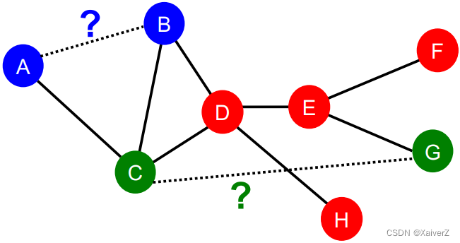
Distance-Based Features

Distance-Based Features

• Key Idea: Shortest-path distance between two nodes (两个节点间最短路径的距离)

  

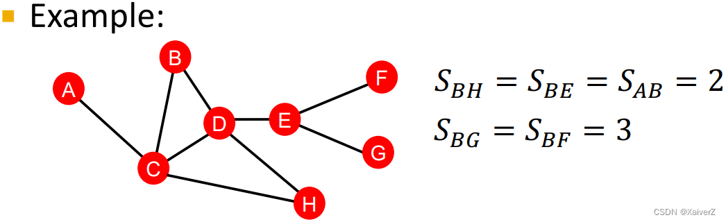
• However, this does not capture the degree of neighborhood overlap (这种方法并没有考虑到两个节点的共同邻居数量)

  • $(B,H)$ has 2 shared neighboring nodes, while $(B,E)$ only have 1 such node

Local Neighborhood Overlap

Local Neighborhood Overlap

• Key Idea: Captures the number of neighboring nodes shared between two nodes $v_1$ and $v_2$ (两节点共同邻居的数量)

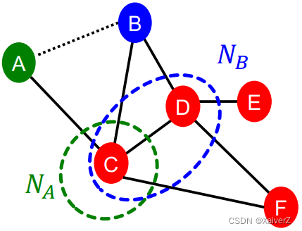
Common Neighbors

Common Neighbors

• Mathematical Form

  $$\left|N\left(v_1\right)\cap N\left(v_2\right)\right|$$

• Example: ∣ N ( A ) ∩ N ( B ) ∣ = ∣ { C } ∣ = 1 |N(A) \cap N(B)|=|\{C\}|=1 ∣N(A)∩N(B)∣=∣{C}∣=1

Jaccard’s Coefficient

Jaccard’s Coefficient

• Mathematical Form

  $$\frac{\left|N\left(v_1\right)\cap N\left(v_2\right)\right|}{\left|N\left(v_1\right)\cup N\left(v_2\right)\right|}$$

• Example: ∣ N ( A ) ∩ N ( B ) ∣ ∣ N ( A ) ∪ N ( B ) ∣ = ∣ { C } ∣ ∣ { C , D } ∣ = 1 2 \frac{|N(A) \cap N(B)|}{|N(A) \cup N(B)|}=\frac{|\{C\}|}{|\{C, D\}|}=\frac{1}{2} ∣N(A)∪N(B)∣∣N(A)∩N(B)∣​=∣{C,D}∣∣{C}∣​=21​

Adamic-Adar Index

Adamic-Adar Index

• Mathematical Form

  $$\sum _{u\in N\left(v_1\right)\cap N\left(v_2\right)}\frac{1}{\log \left(k_u\right)}$$

• Example: $\frac{1}{\log \left(k_C\right)}=\frac{1}{\log 4}$

Global Neighborhood Overlap

Global Neighborhood Overlap

• Limitation of local neighborhood features

  • Metric is always zero if the two nodes do not have any neighbors in common

  

  • However, the two nodes may still potentially be connected in the future

Katz Index

Katz Index

• Key Idea: Count the number of paths of all lengths between a given pair of nodes (计算一对节点间所有不同长度路径的数量)

• Tricks: Use adjacency matrix powers to compute Katz Index

  • $A_{uv}$ specifies #paths of length 1 (direct neighborhood) between $u$ and $v$

  • $A_{uv}^2$ specifies #paths of length 2 (neighbor of neighbor) between $u$ and $v$

  • Inductively, $A_{uv}^l$ specifies #paths of length $l$ between $u$ and $v$

• Katz index between $v_1$ and $v_2$ is calculated as

  $$S_{v_1{v}_2}=\sum _{l=1}^{\infty }{\beta }^l{\mathbf{A}}_{v_1{v}_2}^l$$
  ${\mathbf{A}}_{v_1{v}_2}^l$ is #paths of length $l$ between $v_1$ and $v_2$; $0<\beta <1$ is a discount factor

• Katz index matrix is computed in closed-form (by geometric series of matrices)

  $$\mathbf{S}=\sum _{i=1}^{\infty }{\beta }^i{\mathbf{A}}^i=\underset{={\sum }_{i=0}^{\infty }{\beta }^i{\mathbf{A}}^i}{\underbrace{(\mathbf{I}-\beta \mathbf{A}{)}^{-1}}}-\mathbf{I}$$

Graph-level Features and Graph kernels

Goal: We want features that characterize the structure of an entire graph

Key Idea: Design kernels instead of feature vectors

• Quick Intro to Kernels

  • Kernel $K(G,G^{\prime })\in R$ measures similarity between data

  • Kernel matrix $K=(K(G,G^{\prime }){)}_{G,G^{\prime }}$ must always be positive semidefinite (i.e. has positive eigenvals)

  • There exists a feature representation $\varphi (\cdot )$ such that $K\left(G,G^{\prime }\right)=\varphi (G{)}^{\mathrm{T}}\varphi \left(G^{\prime }\right)$

• Graph Kernel

  Graph Kernels: Measure similarity between two graphs

  • Goal: Design graph feature vector $\varphi (G)$

  • Key Idea: Bag-of-Words (BoW) for a graph, which simply used the word counts as features for documents (no ordering considered)

  • Naive extension to a graph: Regard nodes as words

  • Since both graphs have 4 red nodes, we get the same feature vector for two different graphs…

    

  • And what if we use Bag of node degrees ?

    

• Both Graphlet Kernel and Weisfeiler-Lehman (WL) Kernel use Bag-of-* representation of graph, where * is more sophisticated than node degrees

Graphlet Kernel

Paper : Efficient graphlet kernels for large graph comparison

Graphlet Kernel

• Key Idea: Count the number of different graphlets in a graph

  • The defination of graphlets here is slightly different from node-level features

    • Nodes in graphlets here do not need to be connected (allows for isolated nodes)

    • The graphlets here are not rooted

• Let ${\mathcal{G}}_k=\left(g_1,g_2,\dots ,g_{n_k}\right)$ be a list of graphlets of size $k$

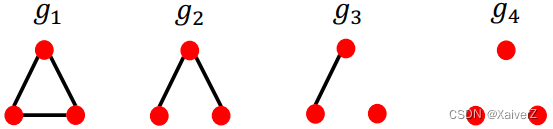
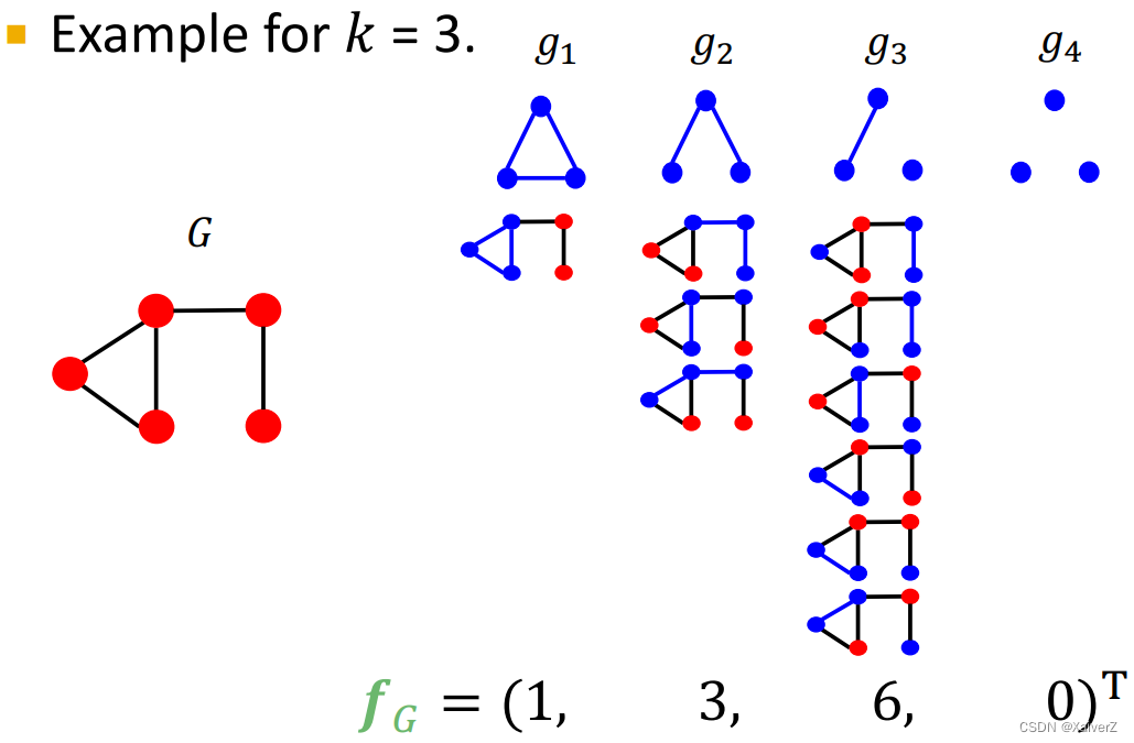
  • For $k=3$, there are 4 graphlets

    

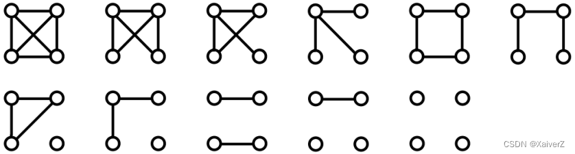
  • For $k=4$, there are 11 graphlets

    

• Given graph $G$, and a graphlet list ${\mathcal{G}}_k=\left(g_1,g_2,\dots ,g_{n_k}\right)$, define the graphlet count vector $f_G\in {\mathbb{R}}^{n_k}$ as

  $${\left({\mathbf{f}}_G\right)}_i=\#\left(g_i\subseteq G\right)\text{ for }i=1,2,\dots ,n_k$$

• Example for $k=3$

  

• Given two graphs, $G$ and $G^{\prime }$, graphlet kernel is computed as

  $$K\left(G,G^{\prime }\right)={\mathbf{f}}_G^{\mathrm{T}}{\mathbf{f}}_{G^{\prime }}$$

  • 若$G$和$G^{\prime }$的节点数不同，那么Graphlet Kernel计算出来的相似度可能存在值偏移（Skew the value），所以这里对特征向量${\mathbf{f}}_G$进行normalize，并使用normalize后的特征向量进行相似度计算

  $${\mathbf{h}}_G=\frac{{\mathbf{f}}_G}{\mathrm{Sum}\left({\mathbf{f}}_G\right)}K\left(G,G^{\prime }\right)={\mathbf{h}}_G{}^{\mathrm{T}}{\mathbf{h}}_{G^{\prime }}$$
  这样一来，${\mathbf{f}}_G$中的每个分量都代表graphlet出现的概率，避免了因图节点数量不同而造成的数据偏移

• Limitation: Counting graphlets is expensive

  • Counting size-k graphlets for a graph with size $n$ by enumeration takes $n^k$

  • This is unavoidable in the worst-case since subgraph isomorphism test (judging whether a graph is a subgraph of another graph) is NP-hard

  • If a graph’s node degree is bounded by $d$, an $O(n{d}^{k-1})$ algorithm exists to count all the graphlets of size $k$

Weisfeiler-Lehman Kernel

Paper : Weisfeiler-Lehman Graph Kernels

Weisfeiler-Lehman Kernel (WL Kernel)

• Goal: Design an efficient graph feature descriptor $\varphi (G)$

• Idea: Use neighborhood structure to iteratively enrich node vocabulary —— Color Refinement

Color Refinement

Color Refinement

• Given: A graph $G$ with a set of nodes $V$

  • Assign an initial color $c^{(0)}(v)$ to each node $v$

  • Iteratively refine node colors by

    $$c^{(k+1)}(v)=\mathrm{HASH}\left(\left\{c^{(k)}(v),{\left\{c^{(k)}(u)\right\}}_{u\in N(v)}\right\}\right)$$
    where $\mathrm{HASH}$ maps different inputs to different colors

  • After $K$ steps of color refinement, $c^{(k)}(v)$ summarizes the structure of K-hop neighborhood

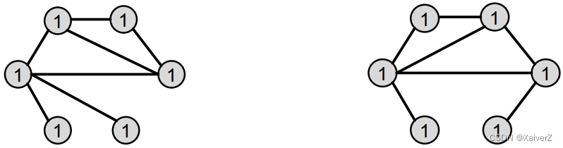
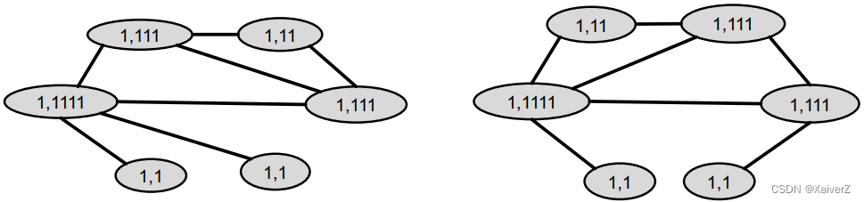
• Example: Use digits for colors

  • Assign initial colors

    

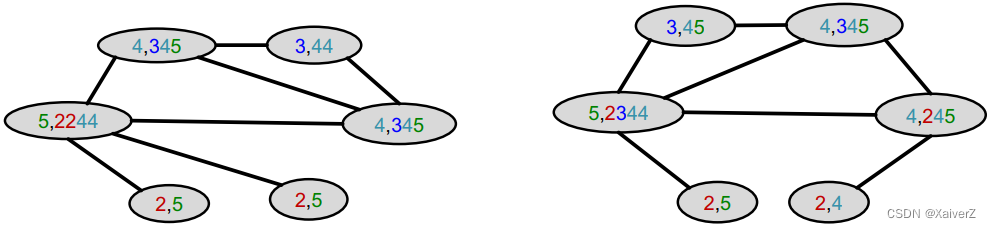
  • Aggregate neighboring colors

    

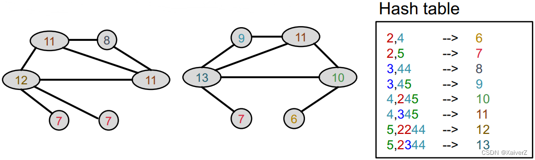
  • Hash aggregated colors

    

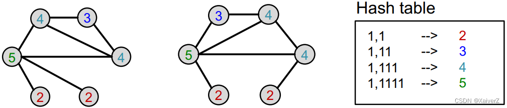
  • Aggregate neighboring colors

    

  • Hash aggregated colors

    

  • After color refinement, WL kernel counts number of nodes with a given color

    

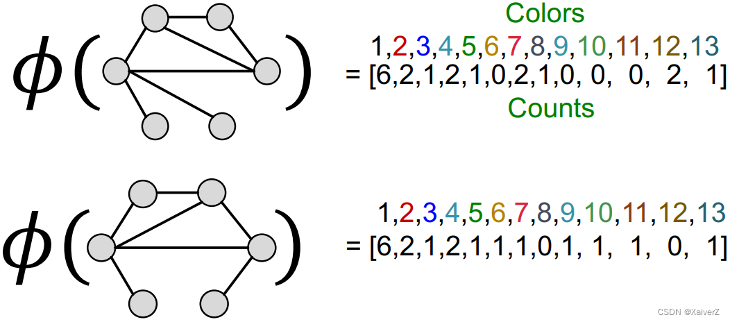
  • The WL kernel value is computed by the inner product of the color count vectors

    

• WL kernel is computationally efficient

  • The time complexity for color refinement at each step is linear in #(edges), since it involves aggregating neighboring colors

  • When computing a kernel value, only colors appeared in the two graphs need to be tracked. Thus, #(colors) is at most the total number of nodes

  • Counting colors takes linear-time w.r.t. #(nodes)

  • In total, time complexity is linear in #(edges)

• The computation manner of WL kernel closely related to Graph Neural Network