


所使用的数据是血友病数据,如有需要,可在主页资源处获取,数据信息如下:
读取数据及数据集区分
数据预处理及区分数据集代码如下(详细预处理说明见上篇文章--随机森林):
import pandas as pd
import numpy as np
hemophilia = pd.read_csv('D:/my_files/data.csv')  #读取数据

#数值变量化为分类变量
hemophilia['hiv']=hemophilia['hiv'].astype(object)
hemophilia['factor']=hemophilia['factor'].astype(object)
new_hemophilia=pd.get_dummies(hemophilia,drop_first=True)
    #drop_first=True--删去一列,如hiv,处理后为两列,都是01表示,但只保留一列就足够表示两种状态
new_data=new_hemophilia
from sklearn.model_selection import train_test_split
x = new_data.drop(['deaths'],axis=1)   #删去标签列
X_train, X_test, y_train, y_test = train_test_split(x, new_data.deaths, test_size=0.3, random_state=0)
    #区分数据集,70%训练集,30%测试集
默认参数XGBoost
先使用默认参数XGBoost进行预测,输出预测均方误差为0.334.
from xgboost import XGBRegressor
from sklearn.model_selection import GridSearchCV
xgb_model = XGBRegressor(random_state=0)  #random_state=0是随机种子数
xgb_model.fit(X_train, y_train)
y_pred = xgb_model.predict(X_test)
print('MSE of xgb: %.3f' %metrics.mean_squared_error(y_test, y_pred))
'''MSE of xgb: 0.334
'''
XGBoost调参
接下来对XGBoost进行调参,XGBoost参数很多,一般对少数参数进行调整就可以得到不错的效果,所以这里只对'max_depth','min_child_weight','gamma'这三个参数进行粗略调参,如果追求更加有效的调参结果,可以对多个参数逐一调参。调参后输出预测均方误差为0.287,已经有所下降,说明模型的预测效果已经得到了提升。
param_grid = {'max_depth':[1,2,3,4,5],
              'min_child_weight':range(10,70,10),
              'gamma':[i*0.01 for i in range(0,20,3)]}
GS = GridSearchCV(xgb_model,param_grid,scoring = 'neg_mean_squared_error',cv=5)
GS.fit(X_train, y_train)
GS.best_params_  #最佳参数组合
   #{'gamma': 0.15, 'max_depth': 3, 'min_child_weight': 68}

xgb_model = XGBRegressor(gamma = 0.15, max_depth = 3, min_child_weight = 60, random_state=0)
xgb_model.fit(X_train, y_train)
y_pred = xgb_model.predict(X_test)
print('MSE of xgb: %.3f' %metrics.mean_squared_error(y_test, y_pred))
'''MSE of xgb: 0.287
'''
XGBoost变量重要性
XGBoost和随机森林都能够输出变量重要性,代码如下:
import matplotlib.pyplot as plt
importances = list(xgb_model.feature_importances_)   #XGBoost
feature_list = list(x.columns)
feature_importances = [(feature, round(importance, 2)) for feature, importance in zip(feature_list, importances)]
feature_importances = sorted(feature_importances, key=lambda x: x[1], reverse=True)
f_list = []
importances_list = []
for i in range(0,8):
    feature = feature_importances[i][0]
    importances_r = feature_importances[i][1]
    f_list.append(feature),importances_list.append(importances_r)
x_values = list(range(len(importances_list)))
plt.figure(figsize=(14, 9))
plt.bar(x_values, importances_list, orientation='vertical')
plt.xticks(x_values, f_list, rotation=25, size =18)
plt.yticks(size =18)
plt.ylabel('Importance',size = 20)
plt.xlabel('Variable',size = 20)
plt.title('XGB Variable Importances',size = 22)
#plt.savefig('D:/files/xgb变量重要性.png', dpi=800)
    #保存图片到指定位置 dpi--分辨率
plt.show()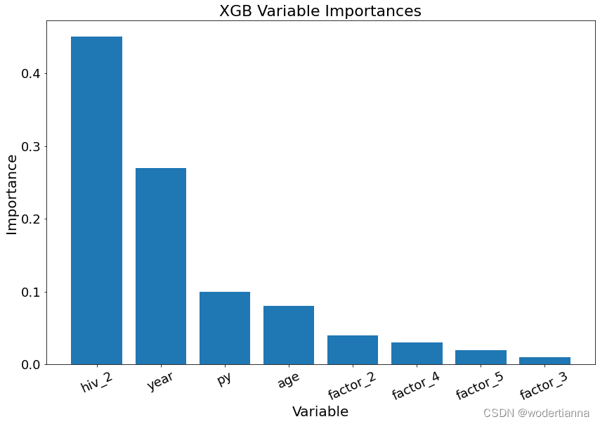
还可以输出图片对比预测结果和真实值的差异,代码及图片如下:
import matplotlib.pyplot as plt
y_test = y_test.reset_index(drop = True)
plt.plot(y_test,color="b",label = 'True')
plt.plot(y_pred,color="r",label = 'Prediction')
plt.xlabel("index")  #x轴命名表示
plt.ylabel("deaths")  #y轴命名表示
plt.title("xgb Comparison between real and perdiction")
plt.legend()  #增加图例
#plt.savefig('D:/my_files/xgb Comparison between real and perdiction.png', dpi = 500) #保存图片
plt.show()  #显示图片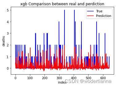


 776
776


 被折叠的 条评论
为什么被折叠?
被折叠的 条评论
为什么被折叠?
 到【灌水乐园】发言


