


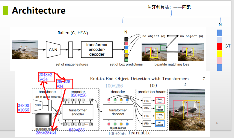
论文标题:End-to-End Object Detection with Transformers
论文官方地址:https://ai.facebook.com/research/publications/end-to-end-object-detection-with-transformers
个人整理的PPT(可编辑),下载地址:DETR学习分享.pptx
一、什么是匈牙利算法
匈牙利匹配算法,是一种典型的一对一的配对算法。一对一的匹配,与之对应的,就是一对多,或多对一的配对算法。也称作 no anchor 操作。
对于Anchor based 、 Anchor free 和 no anchor 的辨析,可以参考这里:【AI面试】Anchor based 、 Anchor free 和 no anchor 的辨析 https://qianlingjun.blog.csdn.net/article/details/129339036在目标检测算法中,预测结果与gt标注结果多对一的典型案例,就是anchor based时候,对推荐的特征框是很多的,但是图像中的标记目标是很少的。对于阳性和阴性案例的分配时候,就采用了IOU 的方式来判别。
- 大于0.7的就是positive,
- 小于0.3的就是negative。
- 即便如此,positive的数量还是相比于标记框数量还是多的,此时的状态就是多对一的。
(上面对于阳性样本和阴性样本的划分,是一个简略的介绍,更详细的可以参考这里:【AI面试】YOLO 如何通过 k-means 得到 anchor boxes的?Yolo、SSD 和 faster rcnn 的正负样本定义)
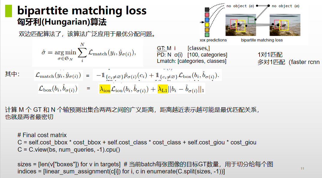
在匈牙利匹配算法组,就是要找到一种一对一的组合方式下,目标是最优的。这里举一个案例:
一个农场主有10名工人,他们分别都有自己擅长的事情,现在需要做5件不同的事情,一个人只能干一件事情。如何分配能够使得最后的工作效率最高呢?
最简单的方式,就是采用遍历的方式,把所有的可能都计算一遍。最后把工作效率最高的一个组合留下来。此时,这种组合就是最优的匹配。
匈牙利匹配算法就是采用这种方式进行的。步骤如下:
- 先定义一个目标任务,怎么判断是最优匹配?比如这里就是误差最小;
- 列举所有的可能,最终找到误差最小的那个组合,就是一一匹配的最优组合形式了。
二、代码
match.py 部分完整代码,如下:
# Copyright (c) Facebook, Inc. and its affiliates. All Rights Reserved
"""
Modules to compute the matching cost and solve the corresponding LSAP.
"""
import torch
from scipy.optimize import linear_sum_assignment
from torch import nn

from util.box_ops import box_cxcywh_to_xyxy, generalized_box_iou


class HungarianMatcher(nn.Module):
    """This class computes an assignment between the targets and the predictions of the network

    For efficiency reasons, the targets don't include the no_object. Because of this, in general,
    there are more predictions than targets. In this case, we do a 1-to-1 matching of the best predictions,
    while the others are un-matched (and thus treated as non-objects).
    """

    def __init__(self, cost_class: float = 1, cost_bbox: float = 1, cost_giou: float = 1):
        """Creates the matcher

        Params:
            cost_class: This is the relative weight of the classification error in the matching cost
            cost_bbox: This is the relative weight of the L1 error of the bounding box coordinates in the matching cost
            cost_giou: This is the relative weight of the giou loss of the bounding box in the matching cost
        """
        super().__init__()
        self.cost_class = cost_class
        self.cost_bbox = cost_bbox
        self.cost_giou = cost_giou
        assert cost_class != 0 or cost_bbox != 0 or cost_giou != 0, "all costs cant be 0"

    @torch.no_grad() # 取消了梯度的产生,不参与回归
    def forward(self, outputs, targets):
        """ Performs the matching

        Params:
            outputs: This is a dict that contains at least these entries:
                 "pred_logits": Tensor of dim [batch_size, num_queries, num_classes] with the classification logits
                 "pred_boxes": Tensor of dim [batch_size, num_queries, 4] with the predicted box coordinates

            targets: This is a list of targets (len(targets) = batch_size), where each target is a dict containing:
                 "labels": Tensor of dim [num_target_boxes] (where num_target_boxes is the number of ground-truth
                           objects in the target) containing the class labels
                 "boxes": Tensor of dim [num_target_boxes, 4] containing the target box coordinates

        Returns:
            A list of size batch_size, containing tuples of (index_i, index_j) where:
                - index_i is the indices of the selected predictions (in order)
                - index_j is the indices of the corresponding selected targets (in order)
            For each batch element, it holds:
                len(index_i) = len(index_j) = min(num_queries, num_target_boxes)
        """
        bs, num_queries = outputs["pred_logits"].shape[:2]

        # We flatten to compute the cost matrices in a batch
        out_prob = outputs["pred_logits"].flatten(0, 1).softmax(-1)  # [batch_size * num_queries, num_classes]
        out_bbox = outputs["pred_boxes"].flatten(0, 1)  # [batch_size * num_queries, 4]

        # Also concat the target labels and boxes
        tgt_ids = torch.cat([v["labels"] for v in targets])
        tgt_bbox = torch.cat([v["boxes"] for v in targets])

        print('0:', out_prob.shape)
        print('1:', out_bbox.shape)

        print('2:', tgt_ids.shape)
        print('3:', tgt_bbox.shape)

        # Compute the classification cost. Contrary to the loss, we don't use the NLL,
        # but approximate it in 1 - proba[target class].
        # The 1 is a constant that doesn't change the matching, it can be ommitted.
        cost_class = -out_prob[:, tgt_ids]  # 1 - proba[target class].  [batch_size * num_queries, target class]
        print('4:', cost_class.shape)
        # print('\n')

        # Compute the L1 cost between boxes,求解正则项,L1范式
        # 这个方法会对每个预测框与GT都进行误差计算。例如预测框N个,GT框M个。结果会有N*M个值(一个batch)
        cost_bbox = torch.cdist(out_bbox, tgt_bbox, p=1)
        print('5:', cost_bbox.shape)

        # Compute the giou cost betwen boxes,省略常熟 1-generalized_box_iou
        cost_giou = -generalized_box_iou(box_cxcywh_to_xyxy(out_bbox), box_cxcywh_to_xyxy(tgt_bbox))
        print('6:', cost_giou.shape)

        # Final cost matrix
        C = self.cost_bbox * cost_bbox + self.cost_class * cost_class + self.cost_giou * cost_giou
        print('7:', C.shape)
        C = C.view(bs, num_queries, -1).cpu()
        print('8:', C.shape)

        sizes = [len(v["boxes"]) for v in targets]  # 当前batch每张图像的目标GT数量,用于切分给每个图
        print('9:', sizes)
        # print('10:', C.split(sizes, -1))
        indices = [linear_sum_assignment(c[i]) for i, c in enumerate(C.split(sizes, -1))]

        for i, c in enumerate(C.split(sizes, -1)):
            import numpy as np
            cost_matrix = np.asarray(c[i])
            # print('cost_matrix:', cost_matrix)
            row_ind, col_ind = linear_sum_assignment(c[i])

            for (row, col) in zip(row_ind, col_ind):
                print(row, col, '***', cost_matrix[row][col])


        print('11:', indices)
        return [(torch.as_tensor(i, dtype=torch.int64), torch.as_tensor(j, dtype=torch.int64)) for i, j in indices]
        # 匈牙利最优匹配,返回匹配索引

def build_matcher(args):
    return HungarianMatcher(cost_class=args.set_cost_class, cost_bbox=args.set_cost_bbox, cost_giou=args.set_cost_giou)
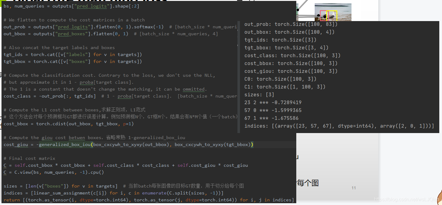
把各阶段显示结果打印出来,查看如下:
0: torch.Size([100, 83])
1: torch.Size([100, 4])
2: torch.Size([3])
3: torch.Size([3, 4])
4: torch.Size([100, 3])
5: torch.Size([100, 3])
6: torch.Size([100, 3])
7: torch.Size([100, 3])
8: torch.Size([1, 100, 3])
9: [3]
10: (tensor([[[ 8.2781e+00,  5.7523e+00,  6.2704e+00],
         [ 4.9576e+00,  6.8206e+00,  5.8613e+00],
         [ 4.3011e+00,  1.1709e+00,  7.6130e+00],
         [ 6.8157e+00,  1.0191e+01,  7.7051e+00],
         [ 5.1331e+00,  2.5986e-01,  9.5993e+00],
         [ 3.6728e+00, -3.1526e-01,  8.6469e+00],
         [ 3.3763e+00,  6.1920e-01,  8.0840e+00],
         [ 4.2639e+00,  3.7820e-01,  8.3531e+00],
         [ 4.9786e+00,  1.4702e+00,  9.3967e+00],
         [ 4.7091e+00,  1.9719e+00,  9.3294e+00],
         [-1.9768e-01,  5.2733e+00,  4.0208e+00],
         [ 7.9992e+00,  5.5239e+00,  6.2364e+00],
         [-6.9660e-02,  4.1440e+00,  4.9423e+00],
         [ 3.6899e+00,  8.7728e+00,  2.2498e-01],
         [ 8.3986e-01,  5.0391e+00,  4.6867e+00],
         [ 5.2078e+00, -1.0942e+00,  9.9988e+00],
         [ 9.2502e+00,  6.9210e+00,  9.6557e+00],
         [ 6.6826e+00,  1.0023e+01,  7.5727e+00],
         [-4.2688e-01,  5.6021e+00,  3.7218e+00],
         [ 1.5247e+00,  4.2876e+00,  6.6519e+00],
         [-4.5765e-01,  5.3721e+00,  4.0550e+00],
         [-1.0363e-01,  5.3039e+00,  3.8190e+00],
         [ 7.0395e-01,  5.4264e+00,  3.7965e+00],
         [ 4.5934e+00,  9.4687e+00, -9.1822e-01],
         [ 6.6833e+00,  1.0135e+01,  7.5300e+00],
         [-4.8056e-01,  5.0123e+00,  4.2394e+00],
         [ 2.6458e-01,  5.1980e+00,  4.0117e+00],
         [ 4.1776e+00, -2.8836e-01,  8.6328e+00],
         [ 6.6063e+00,  9.5719e+00,  7.3849e+00],
         [ 6.2134e+00,  3.5192e+00,  7.1582e+00],
         [ 7.1327e+00,  4.5764e+00,  6.3685e+00],
         [ 3.7398e+00, -9.6579e-02,  8.5241e+00],
         [ 6.8127e+00,  4.1113e+00,  6.5262e+00],
         [ 3.5170e+00,  8.8692e+00,  3.4571e+00],
         [ 1.5750e-02,  4.7749e+00,  4.2767e+00],
         [ 3.8504e+00,  6.3830e-01,  8.3046e+00],
         [ 3.2140e+00,  8.3388e+00,  6.9667e-01],
         [ 4.1912e+00,  8.4101e-01,  8.4362e+00],
         [ 3.5930e+00,  1.1387e-01,  8.3090e+00],
         [ 3.6005e+00,  8.4123e+00,  4.9653e+00],
         [ 3.3979e+00,  8.6321e+00,  3.6201e+00],
         [ 8.2190e-01,  3.8224e+00,  5.8881e+00],
         [ 1.0869e+00,  3.9131e+00,  6.9495e+00],
         [ 4.0383e+00, -1.6680e-01,  8.6249e+00],
         [ 4.5527e+00,  1.3161e+00,  8.0127e+00],
         [ 4.8717e+00, -1.1607e+00,  9.6060e+00],
         [-2.3139e-01,  5.9623e+00,  3.7352e+00],
         [-5.2189e-01,  5.1185e+00,  4.1926e+00],
         [ 5.1255e+00, -1.0225e+00,  9.5479e+00],
         [ 4.0998e+00,  8.8282e-01,  8.1521e+00],
         [ 7.9094e+00,  5.9065e+00,  9.1802e+00],
         [ 5.6728e-01,  4.0475e+00,  6.3995e+00],
         [ 5.6560e+00,  2.6218e+00,  6.4698e+00],
         [ 4.0612e+00,  1.8517e-01,  8.8067e+00],
         [ 8.0742e+00,  5.5891e+00,  6.2239e+00],
         [ 4.0400e+00, -4.1363e-01,  8.6222e+00],
         [ 6.4105e+00,  3.6744e+00,  6.7804e+00],
         [-1.7385e+00,  4.9004e+00,  4.6942e+00],
         [ 3.7932e+00, -3.4077e-01,  8.6290e+00],
         [ 1.5052e+00,  4.1979e+00,  6.7877e+00],
         [ 4.9204e+00,  1.4836e-01,  9.7124e+00],
         [ 4.0792e+00, -8.9709e-01,  8.9150e+00],
         [ 1.2695e+00,  6.2007e+00,  6.3281e+00],
         [ 4.7756e+00, -2.6407e-02,  9.4340e+00],
         [ 6.8410e+00,  1.0208e+01,  7.6384e+00],
         [ 3.7301e+00,  4.3986e-01,  8.0444e+00],
         [ 4.9536e+00,  5.4823e-01,  9.4097e+00],
         [ 4.6248e+00, -1.5043e+00,  9.4438e+00],
         [ 4.8150e+00,  1.5749e+00,  8.2575e+00],
         [ 2.6885e+00,  7.9073e+00,  1.2976e+00],
         [ 4.5642e+00,  9.2036e+00,  5.3550e+00],
         [ 5.4012e+00, -5.6389e-01,  1.0175e+01],
         [ 4.2466e-01,  3.5950e+00,  5.6307e+00],
         [ 4.5491e-02,  5.9585e+00,  3.3820e+00],
         [-5.2628e-01,  5.4329e+00,  4.0332e+00],
         [-4.2191e-01,  5.0971e+00,  4.0838e+00],
         [ 4.4857e+00,  5.5204e-01,  8.3841e+00],
         [ 8.6591e+00,  6.1527e+00,  6.5773e+00],
         [ 4.1859e+00,  1.0231e+00,  8.2301e+00],
         [ 4.3173e+00,  1.5263e+00,  8.0855e+00],
         [ 1.9756e+00,  7.3597e+00,  1.8068e+00],
         [ 3.7020e+00, -1.5050e-03,  8.4148e+00],
         [ 1.2558e+00,  6.2132e+00,  2.9544e+00],
         [ 5.5785e+00,  8.5805e+00,  6.9275e+00],
         [ 4.4306e+00,  1.2772e+00,  7.9827e+00],
         [ 6.9211e-01,  6.3655e+00,  2.7999e+00],
         [ 4.4060e+00,  9.3261e+00, -1.0840e+00],
         [-3.4285e-01,  3.9853e+00,  5.7059e+00],
         [ 4.3454e+00,  4.4445e+00,  9.2292e+00],
         [-1.5630e+00,  4.9668e+00,  4.5768e+00],
         [-1.2383e+00,  4.4616e+00,  4.9227e+00],
         [ 1.6393e-01,  4.6841e+00,  4.3523e+00],
         [-5.9907e-01,  5.0048e+00,  4.3742e+00],
         [ 5.1124e+00,  6.9615e+00,  6.0210e+00],
         [ 3.0988e-03,  6.2910e+00,  3.5968e+00],
         [-4.8344e-01,  4.9876e+00,  4.4395e+00],
         [ 5.1149e+00,  1.9913e+00,  7.9950e+00],
         [ 5.6246e+00,  8.8102e+00,  7.0050e+00],
         [ 2.6130e-01,  3.6337e+00,  5.7934e+00],
         [ 5.5709e+00,  8.9151e+00,  6.7141e+00]]]),)
cost_matrix: [[ 8.2780924e+00  5.7523308e+00  6.2704163e+00]
 [ 4.9575653e+00  6.8206110e+00  5.8613491e+00]
 [ 4.3011103e+00  1.1708755e+00  7.6129541e+00]
 [ 6.8156848e+00  1.0191437e+01  7.7051115e+00]
 [ 5.1331429e+00  2.5985980e-01  9.5993195e+00]
 [ 3.6727586e+00 -3.1525683e-01  8.6469116e+00]
 [ 3.3762672e+00  6.1919785e-01  8.0840225e+00]
 [ 4.2639432e+00  3.7819684e-01  8.3531294e+00]
 [ 4.9785528e+00  1.4702234e+00  9.3966799e+00]
 [ 4.7090969e+00  1.9718820e+00  9.3293982e+00]
 [-1.9767678e-01  5.2733393e+00  4.0208311e+00]
 [ 7.9992228e+00  5.5239344e+00  6.2364326e+00]
 [-6.9660187e-02  4.1440396e+00  4.9423199e+00]
 [ 3.6898577e+00  8.7727966e+00  2.2497982e-01]
 [ 8.3986056e-01  5.0390706e+00  4.6867170e+00]
 [ 5.2078104e+00 -1.0942475e+00  9.9988441e+00]
 [ 9.2502470e+00  6.9209762e+00  9.6557140e+00]
 [ 6.6826372e+00  1.0023033e+01  7.5726542e+00]
 [-4.2687911e-01  5.6021390e+00  3.7218261e+00]
 [ 1.5246817e+00  4.2875733e+00  6.6519294e+00]
 [-4.5764512e-01  5.3720751e+00  4.0549679e+00]
 [-1.0362893e-01  5.3039198e+00  3.8189650e+00]
 [ 7.0395356e-01  5.4264174e+00  3.7965493e+00]
 [ 4.5933971e+00  9.4687033e+00 -9.1822195e-01]
 [ 6.6832952e+00  1.0134920e+01  7.5299850e+00]
 [-4.8055774e-01  5.0122609e+00  4.2393503e+00]
 [ 2.6457596e-01  5.1979795e+00  4.0117393e+00]
 [ 4.1775527e+00 -2.8836286e-01  8.6328087e+00]
 [ 6.6063323e+00  9.5719442e+00  7.3848906e+00]
 [ 6.2134027e+00  3.5191741e+00  7.1582074e+00]
 [ 7.1326599e+00  4.5764084e+00  6.3685322e+00]
 [ 3.7398467e+00 -9.6579432e-02  8.5240564e+00]
 [ 6.8126822e+00  4.1112809e+00  6.5261931e+00]
 [ 3.5170491e+00  8.8692226e+00  3.4571378e+00]
 [ 1.5750408e-02  4.7749467e+00  4.2767425e+00]
 [ 3.8504438e+00  6.3830268e-01  8.3045692e+00]
 [ 3.2139552e+00  8.3388023e+00  6.9667470e-01]
 [ 4.1911783e+00  8.4101266e-01  8.4362345e+00]
 [ 3.5929587e+00  1.1386955e-01  8.3090458e+00]
 [ 3.6005147e+00  8.4122725e+00  4.9652863e+00]
 [ 3.3979454e+00  8.6320591e+00  3.6200943e+00]
 [ 8.2189524e-01  3.8224022e+00  5.8880587e+00]
 [ 1.0868909e+00  3.9131203e+00  6.9494729e+00]
 [ 4.0383496e+00 -1.6679776e-01  8.6248922e+00]
 [ 4.5527411e+00  1.3160551e+00  8.0127211e+00]
 [ 4.8717475e+00 -1.1606574e+00  9.6059589e+00]
 [-2.3138726e-01  5.9623160e+00  3.7351766e+00]
 [-5.2189153e-01  5.1185379e+00  4.1925898e+00]
 [ 5.1254988e+00 -1.0224745e+00  9.5478582e+00]
 [ 4.0997610e+00  8.8282138e-01  8.1520863e+00]
 [ 7.9093728e+00  5.9065194e+00  9.1801624e+00]
 [ 5.6727898e-01  4.0474801e+00  6.3994970e+00]
 [ 5.6560211e+00  2.6217759e+00  6.4698277e+00]
 [ 4.0612087e+00  1.8516517e-01  8.8067341e+00]
 [ 8.0741739e+00  5.5890713e+00  6.2239499e+00]
 [ 4.0400124e+00 -4.1362917e-01  8.6222038e+00]
 [ 6.4105182e+00  3.6743789e+00  6.7803993e+00]
 [-1.7385412e+00  4.9003649e+00  4.6941576e+00]
 [ 3.7932222e+00 -3.4077275e-01  8.6289921e+00]
 [ 1.5052190e+00  4.1978951e+00  6.7876673e+00]
 [ 4.9203916e+00  1.4835656e-01  9.7123594e+00]
 [ 4.0792198e+00 -8.9708799e-01  8.9150419e+00]
 [ 1.2695322e+00  6.2007360e+00  6.3281250e+00]
 [ 4.7756453e+00 -2.6406884e-02  9.4340038e+00]
 [ 6.8410158e+00  1.0207616e+01  7.6383772e+00]
 [ 3.7301140e+00  4.3985701e-01  8.0444126e+00]
 [ 4.9535618e+00  5.4822862e-01  9.4097462e+00]
 [ 4.6247811e+00 -1.5043023e+00  9.4437799e+00]
 [ 4.8150125e+00  1.5749331e+00  8.2575169e+00]
 [ 2.6885109e+00  7.9073000e+00  1.2975867e+00]
 [ 4.5641971e+00  9.2036409e+00  5.3550172e+00]
 [ 5.4011717e+00 -5.6389362e-01  1.0175209e+01]
 [ 4.2465532e-01  3.5949950e+00  5.6307044e+00]
 [ 4.5490503e-02  5.9585238e+00  3.3820138e+00]
 [-5.2628189e-01  5.4329481e+00  4.0332346e+00]
 [-4.2191225e-01  5.0970836e+00  4.0838089e+00]
 [ 4.4857378e+00  5.5203629e-01  8.3840704e+00]
 [ 8.6590862e+00  6.1527267e+00  6.5773430e+00]
 [ 4.1858683e+00  1.0230734e+00  8.2301025e+00]
 [ 4.3172894e+00  1.5262530e+00  8.0854750e+00]
 [ 1.9755765e+00  7.3597250e+00  1.8067718e+00]
 [ 3.7019567e+00 -1.5050173e-03  8.4148455e+00]
 [ 1.2558209e+00  6.2131724e+00  2.9543672e+00]
 [ 5.5785089e+00  8.5805359e+00  6.9275179e+00]
 [ 4.4305744e+00  1.2771857e+00  7.9826665e+00]
 [ 6.9210845e-01  6.3654633e+00  2.7999129e+00]
 [ 4.4059572e+00  9.3260632e+00 -1.0840294e+00]
 [-3.4284663e-01  3.9852719e+00  5.7058821e+00]
 [ 4.3453894e+00  4.4444699e+00  9.2292423e+00]
 [-1.5629959e+00  4.9667954e+00  4.5767879e+00]
 [-1.2383235e+00  4.4615502e+00  4.9226542e+00]
 [ 1.6393489e-01  4.6840563e+00  4.3522577e+00]
 [-5.9907275e-01  5.0048246e+00  4.3741856e+00]
 [ 5.1123734e+00  6.9614697e+00  6.0210080e+00]
 [ 3.0988455e-03  6.2910314e+00  3.5968068e+00]
 [-4.8343736e-01  4.9875731e+00  4.4395008e+00]
 [ 5.1148849e+00  1.9913349e+00  7.9949999e+00]
 [ 5.6245937e+00  8.8101625e+00  7.0049658e+00]
 [ 2.6129830e-01  3.6337457e+00  5.7934051e+00]
 [ 5.5708518e+00  8.9150972e+00  6.7141314e+00]]
57 0 *** -1.7385412
67 1 *** -1.5043023
86 2 *** -1.0840294
11: [(array([57, 67, 86], dtype=int64), array([0, 1, 2]))]
上述直观到一张图看,如下这样:
其中核心部分,linear_sum_assignment的定义如下:
# Wrapper for the shortest augmenting path algorithm for solving the
# rectangular linear sum assignment problem.  The original code was an
# implementation of the Hungarian algorithm (Kuhn-Munkres) taken from
# scikit-learn, based on original code by Brian Clapper and adapted to NumPy
# by Gael Varoquaux. Further improvements by Ben Root, Vlad Niculae, Lars
# Buitinck, and Peter Larsen.
#
# Copyright (c) 2008 Brian M. Clapper <bmc@clapper.org>, Gael Varoquaux
# Author: Brian M. Clapper, Gael Varoquaux
# License: 3-clause BSD

import numpy as np
from . import _lsap_module


def linear_sum_assignment(cost_matrix, maximize=False):
    """Solve the linear sum assignment problem.

    The linear sum assignment problem is also known as minimum weight matching
    in bipartite graphs. A problem instance is described by a matrix C, where
    each C[i,j] is the cost of matching vertex i of the first partite set
    (a "worker") and vertex j of the second set (a "job"). The goal is to find
    a complete assignment of workers to jobs of minimal cost.

    Formally, let X be a boolean matrix where :math:`X[i,j] = 1` iff row i is
    assigned to column j. Then the optimal assignment has cost

    .. math::
        \\min \\sum_i \\sum_j C_{i,j} X_{i,j}

    where, in the case where the matrix X is square, each row is assigned to
    exactly one column, and each column to exactly one row.

    This function can also solve a generalization of the classic assignment
    problem where the cost matrix is rectangular. If it has more rows than
    columns, then not every row needs to be assigned to a column, and vice
    versa.

    Parameters
    ----------
    cost_matrix : array
        The cost matrix of the bipartite graph.

    maximize : bool (default: False)
        Calculates a maximum weight matching if true.

    Returns
    -------
    row_ind, col_ind : array
        An array of row indices and one of corresponding column indices giving
        the optimal assignment. The cost of the assignment can be computed
        as ``cost_matrix[row_ind, col_ind].sum()``. The row indices will be
        sorted; in the case of a square cost matrix they will be equal to
        ``numpy.arange(cost_matrix.shape[0])``.

    Notes
    -----
    .. versionadded:: 0.17.0

    References
    ----------

    1. https://en.wikipedia.org/wiki/Assignment_problem

    2. DF Crouse. On implementing 2D rectangular assignment algorithms.
       *IEEE Transactions on Aerospace and Electronic Systems*,
       52(4):1679-1696, August 2016, https://doi.org/10.1109/TAES.2016.140952

    Examples
    --------
    >>> cost = np.array([[4, 1, 3], [2, 0, 5], [3, 2, 2]])
    >>> from scipy.optimize import linear_sum_assignment
    >>> row_ind, col_ind = linear_sum_assignment(cost)
    >>> col_ind
    array([1, 0, 2])
    >>> cost[row_ind, col_ind].sum()
    5
    """
    cost_matrix = np.asarray(cost_matrix)
    if len(cost_matrix.shape) != 2:
        raise ValueError("expected a matrix (2-d array), got a %r array"
                         % (cost_matrix.shape,))

    if not (np.issubdtype(cost_matrix.dtype, np.number) or
            cost_matrix.dtype == np.dtype(np.bool)):
        raise ValueError("expected a matrix containing numerical entries, got %s"
                         % (cost_matrix.dtype,))

    if maximize:
        cost_matrix = -cost_matrix

    if np.any(np.isneginf(cost_matrix) | np.isnan(cost_matrix)):
        raise ValueError("matrix contains invalid numeric entries")

    cost_matrix = cost_matrix.astype(np.double)
    a = np.arange(np.min(cost_matrix.shape))

    # The algorithm expects more columns than rows in the cost matrix.
    if cost_matrix.shape[1] < cost_matrix.shape[0]:
        b = _lsap_module.calculate_assignment(cost_matrix.T)
        indices = np.argsort(b)
        return (b[indices], a[indices])
    else:
b = _lsap_module.calculate_assignme看完这个,就觉得他好像就干了一件事:取最小的值,就是下面这段:
 cost_matrix = cost_matrix.astype(np.double)
 a = np.arange(np.min(cost_matrix.shape))
用它给的这个栗子看看,输入代码是这样的:
import numpy as np
cost = np.array([[4, 1, 3],
                 [2, 0, 5],
                 [3, 2, 2]])
from scipy.optimize import linear_sum_assignment
row_ind, col_ind = linear_sum_assignment(cost)
print(row_ind, col_ind)
for (row, col) in zip(row_ind, col_ind):
    print(row, col, '***', cost[row][col])
打印的结果如下:(按行取最小值)
[0 1 2] [1 0 2]
0 1 *** 1
1 0 *** 2
2 2 *** 2
三、总结
总结一下,匈牙利Hungarian算法在这里显得很蛮力。为了将预测的框,与标注的框找到1对1的最佳匹配,直接将预测的框M个,与标注的框N个,直接进行一一对应,组成一个M行N例的一个cost矩阵,其中每一个cost[m][n]就是一中组合对应形式。
最后,再按标注的N列,取出N个最优的预测值,这样构成预测与标注的一一对应,记为最佳匹配。


 9万+
9万+

 被折叠的 条评论
为什么被折叠?
被折叠的 条评论
为什么被折叠?
 到【灌水乐园】发言


