


推荐阅读列表:
本文以MNIST数据集为例,从零构建扩散模型,具体会涉及到如下知识点:
- 退化过程(向数据中添加噪声)
- 构建一个简单的UNet模型
- 训练扩散模型
- 采样过程分析
下面介绍具体的实现过程:
一、环境配置&python包的导入
最好有GPU环境,比如公司的GPU集群或者Google Colab,下面是代码实现:
# 安装diffusers库!pip install -q diffusers# 导入所需要的包import torchimport torchvisionfrom torch import nnfrom torch.nn import functional as Ffrom torch.utils.data import DataLoaderfrom diffusers import DDPMScheduler, UNet2DModelfrom matplotlib import pyplot as pltdevice = torch.device("cuda" if torch.cuda.is_available() else "cpu")print(f'Using device: {device}')
# 输出Using device: cuda
此时会输出运行环境是GPU还是CPU
二、加载MNIST数据集
MNIST数据集是一个小数据集,存储的是0-9手写数字字体,每张图片都28X28的灰度图片,每个像素的取值范围是[0,1],下面加载该数据集,并展示部分数据:
dataset = torchvision.datasets.MNIST(root="mnist/", train=True, download=True, transform=torchvision.transforms.ToTensor())train_dataloader = DataLoader(dataset, batch_size=8, shuffle=True)x, y = next(iter(train_dataloader))print('Input shape:', x.shape)print('Labels:', y)plt.imshow(torchvision.utils.make_grid(x)[0], cmap='Greys');
# 输出Input shape: torch.Size([8, 1, 28, 28])Labels: tensor([7, 8, 4, 2, 3, 6, 0, 2])

三、扩散模型的退化过程
所谓退化过程,其实就是对输入数据加入噪声的过程,由于MNIST数据集的像素范围在[0,1],那么我们加入噪声也需要保持在相同的范围,这样我们可以很容易的把输入数据与噪声进行混合,代码如下:
def corrupt(x, amount):"""Corrupt the input `x` by mixing it with noise according to `amount`"""noise = torch.rand_like(x)amount = amount.view(-1, 1, 1, 1) # Sort shape so broadcasting worksreturn x*(1-amount) + noise*amount
接下来,我们看一下逐步加噪的效果,代码如下:
# Plotting the input datafig, axs = plt.subplots(2, 1, figsize=(12, 5))axs[0].set_title('Input data')axs[0].imshow(torchvision.utils.make_grid(x)[0], cmap='Greys')# Adding noiseamount = torch.linspace(0, 1, x.shape[0]) # Left to right -> more corruptionnoised_x = corrupt(x, amount)# Plottinf the noised versionaxs[1].set_title('Corrupted data (-- amount increases -->)')axs[1].imshow(torchvision.utils.make_grid(noised_x)[0], cmap='Greys');

从上图可以看出,从左到右加入的噪声逐步增多,当噪声量接近1时,数据看起来像纯粹的随机噪声。
四、构建一个简单的UNet模型
UNet模型与自编码器有异曲同工之妙,UNet最初是用于完成医学图像中分割任务的,网络结构如下所示:

代码如下:
class BasicUNet(nn.Module):"""A minimal UNet implementation."""def __init__(self, in_channels=1, out_channels=1):super().__init__()self.down_layers = torch.nn.ModuleList([nn.Conv2d(in_channels, 32, kernel_size=5, padding=2),nn.Conv2d(32, 64, kernel_size=5, padding=2),nn.Conv2d(64, 64, kernel_size=5, padding=2),])self.up_layers = torch.nn.ModuleList([nn.Conv2d(64, 64, kernel_size=5, padding=2),nn.Conv2d(64, 32, kernel_size=5, padding=2),nn.Conv2d(32, out_channels, kernel_size=5, padding=2),])self.act = nn.SiLU() # The activation functionself.downscale = nn.MaxPool2d(2)self.upscale = nn.Upsample(scale_factor=2)def forward(self, x):h = []for i, l in enumerate(self.down_layers):x = self.act(l(x)) # Through the layer and the activation functionif i < 2: # For all but the third (final) down layer:h.append(x) # Storing output for skip connectionx = self.downscale(x) # Downscale ready for the next layerfor i, l in enumerate(self.up_layers):if i > 0: # For all except the first up layerx = self.upscale(x) # Upscalex += h.pop() # Fetching stored output (skip connection)x = self.act(l(x)) # Through the layer and the activation functionreturn x
我们来检验一下模型输入输出的shape变化是否符合预期,代码如下:
net = BasicUNet()x = torch.rand(8, 1, 28, 28)net(x).shape
# 输出torch.Size([8, 1, 28, 28])
再来看一下模型的参数量,代码如下:
sum([p.numel() for p in net.parameters()])# 输出309057
至此,已经完成数据加载和UNet模型构建,当然UNet模型的结构可以有不同的设计。
五、扩散模型训练
扩散模型应该学习什么?其实有很多不同的目标,比如学习噪声,我们先以一个简单的例子开始,输入数据为带噪声的MNIST数据,扩散模型应该输出对应的最佳数字预测,因此学习的目标是预测值与真实值的MSE,训练代码如下:
# Dataloader (you can mess with batch size)batch_size = 128train_dataloader = DataLoader(dataset, batch_size=batch_size, shuffle=True)# How many runs through the data should we do?n_epochs = 3# Create the networknet = BasicUNet()net.to(device)# Our loss finctionloss_fn = nn.MSELoss()# The optimizeropt = torch.optim.Adam(net.parameters(), lr=1e-3)# Keeping a record of the losses for later viewinglosses = []# The training loopfor epoch in range(n_epochs):for x, y in train_dataloader:# Get some data and prepare the corrupted versionx = x.to(device) # Data on the GPUnoise_amount = torch.rand(x.shape[0]).to(device) # Pick random noise amountsnoisy_x = corrupt(x, noise_amount) # Create our noisy x# Get the model predictionpred = net(noisy_x)# Calculate the lossloss = loss_fn(pred, x) # How close is the output to the true 'clean' x?# Backprop and update the params:opt.zero_grad()loss.backward()opt.step()# Store the loss for laterlosses.append(loss.item())# Print our the average of the loss values for this epoch:avg_loss = sum(losses[-len(train_dataloader):])/len(train_dataloader)print(f'Finished epoch {epoch}. Average loss for this epoch: {avg_loss:05f}')# View the loss curveplt.plot(losses)plt.ylim(0, 0.1);
# 输出Finished epoch 0. Average loss for this epoch: 0.024689Finished epoch 1. Average loss for this epoch: 0.019226Finished epoch 2. Average loss for this epoch: 0.017939
训练过程的loss曲线如下图所示:

六、扩散模型效果评估
我们选取一部分数据来评估一下模型的预测效果,代码如下:
#@markdown Visualizing model predictions on noisy inputs:# Fetch some datax, y = next(iter(train_dataloader))x = x[:8] # Only using the first 8 for easy plotting# Corrupt with a range of amountsamount = torch.linspace(0, 1, x.shape[0]) # Left to right -> more corruptionnoised_x = corrupt(x, amount)# Get the model predictionswith torch.no_grad():preds = net(noised_x.to(device)).detach().cpu()# Plotfig, axs = plt.subplots(3, 1, figsize=(12, 7))axs[0].set_title('Input data')axs[0].imshow(torchvision.utils.make_grid(x)[0].clip(0, 1), cmap='Greys')axs[1].set_title('Corrupted data')axs[1].imshow(torchvision.utils.make_grid(noised_x)[0].clip(0, 1), cmap='Greys')axs[2].set_title('Network Predictions')axs[2].imshow(torchvision.utils.make_grid(preds)[0].clip(0, 1), cmap='Greys');
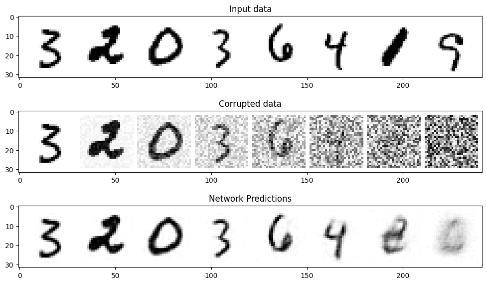
从上图可以看出,对于噪声量较低的输入,模型的预测效果是很不错的,当amount=1时,模型的输出接近整个数据集的均值,这正是扩散模型的工作原理。
Note:我们的训练并不太充分,读者可以尝试不同的超参数来优化模型。


 3503
3503


 被折叠的 条评论
为什么被折叠?
被折叠的 条评论
为什么被折叠?
 到【灌水乐园】发言


