Swin Transformer V2 的改进和源码分析

Swin Transformer V2 论文地址

Swin Transformer V2 源码地址

对 Swin Transformer 还不太熟悉的可以先移步到我的

Swin Transformer源码分析

就如论文标题

Swin Transformer V2: Scaling Up Capacity and Resolution  

一个字就是大 模型大尺寸大

如论文所述

 

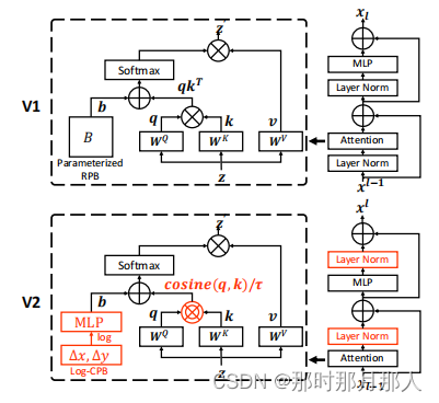
To better scale up model capacity and window resolution, several adaptions are made on the original Swin Transformer architecture (V1): 1) A res-post-norm to replace the previous pre norm confifiguration; 2) A scaled cosine attention to replace the original dot product attention ; 3) A log-spaced continuous relative position bias approach to replace the previous parameterized approach. Adaptions 1) and 2) make it easier for the model to scale up capacity. Adaption 3) makes the model to be transferred more effectively across window resolutions. The adapted architecture is named Swin Transformer V2.

 做了三个主要变化:

1. res-post-norm  简单来说norm层后置了。  以前是  Attention + Layer Norm 变成 Layer Norm + Attention。前馈神经网络的 Layer Norm也后置了。至于原因是因为 模型变大了 每层输出变得不稳定，输出逐层放大 ，导致模型难以收敛。所以 Layer Norm 层后置为了让每层输出值稳定。

2. A scaled cosine attention to replace the original dot product attention 这更好理解了 原来的点乘 q * k.T 变成了 cosine 运算   (q * k) /  || q || * || k || ，并引入了一个超参数 τ 来对值进行缩放，进一步控制输出，注意：超参数 τ 每层block不共享 。

3. A log-spaced continuous relative position bias approach to replace the previous parameterized approach. 提出了一个新的相对编码计算方式

 

 第一点: Layer Norm 后置

class SwinTransformerBlock(nn.Module):
       """
            上述代码略
       """

       # 从这里可以看出 两个 layer norm 层都后置了
        x = shortcut + self.drop_path(self.norm1(x))

        # FFN
        x = x + self.drop_path(self.norm2(self.mlp(x)))

        return x

第二点 点乘变成了 cosine 相似度计算

q, k, v = qkv[0], qkv[1], qkv[2]  # make torchscript happy (cannot use tensor as tuple)

# cosine attention
attn = (F.normalize(q, dim=-1) @ F.normalize(k, dim=-1).transpose(-2, -1))
logit_scale = torch.clamp(self.logit_scale, max=torch.log(torch.tensor(1. / 0.01))).exp()
attn = attn * logit_scale

# mlp to generate continuous relative position bias
# 为了生成一个连续的相对位置 bias
self.cpb_mlp = nn.Sequential(nn.Linear(2, 512, bias=True),
                             nn.ReLU(inplace=True),
                             nn.Linear(512, num_heads, bias=False))

# get relative_coords_table
# 生成log连续的相对位置表
relative_coords_h = torch.arange(-(self.window_size[0] - 1), self.window_size[0], dtype=torch.float32)
relative_coords_w = torch.arange(-(self.window_size[1] - 1), self.window_size[1], dtype=torch.float32)
relative_coords_table = torch.stack(
    torch.meshgrid([relative_coords_h,
                    relative_coords_w])).permute(1, 2, 0).contiguous().unsqueeze(0)  # 1, 2*Wh-1, 2*Ww-1, 2
# 进行归一化到 -1 ~ 1
if pretrained_window_size[0] > 0:
    relative_coords_table[:, :, :, 0] /= (pretrained_window_size[0] - 1)
    relative_coords_table[:, :, :, 1] /= (pretrained_window_size[1] - 1)
else:
    relative_coords_table[:, :, :, 0] /= (self.window_size[0] - 1)
    relative_coords_table[:, :, :, 1] /= (self.window_size[1] - 1)
# 将值 normalize to -8, 8
relative_coords_table *= 8  # normalize to -8, 8
relative_coords_table = torch.sign(relative_coords_table) * torch.log2(
    torch.abs(relative_coords_table) + 1.0) / np.log2(8)

self.register_buffer("relative_coords_table", relative_coords_table)

# get pair-wise relative position index for each token inside the window
# 下面是得到 window内 的相对位置坐标
coords_h = torch.arange(self.window_size[0])
coords_w = torch.arange(self.window_size[1])
coords = torch.stack(torch.meshgrid([coords_h, coords_w]))  # 2, Wh, Ww
coords_flatten = torch.flatten(coords, 1)  # 2, Wh*Ww
# 下面两行其实也就是将数据展平后 广播后相减 得到相对坐标
relative_coords = coords_flatten[:, :, None] - coords_flatten[:, None, :]  # 2, Wh*Ww, Wh*Ww
relative_coords = relative_coords.permute(1, 2, 0).contiguous()  # Wh*Ww, Wh*Ww, 2
# 但是上面的相对坐标和定义的 relative_position_bias_table还对应不上 relative_coords 取值范围 (-w + 1) ~ (w - 1)
# 所以在dim=[1, 2] 维度 才加上 self.window_size[0] - 1 取值范围 变成 0 ~ (2w - 2)
relative_coords[:, :, 0] += self.window_size[0] - 1  # shift to start from 0
relative_coords[:, :, 1] += self.window_size[1] - 1
# 最后在 dim=2 的维度上 乘以 2w - 1 所以在这个维度上取值范围为 0 ~  (2w - 2) * (2w - 1) = (2w - 1)**2 - (2w - 1)
relative_coords[:, :, 0] *= 2 * self.window_size[1] - 1
# 最后求和后得到的相对坐标范围 0 ~ (2w - 1)**2 - (2w - 1) + (2w - 2) = (2w - 1)**2 - 1
# OKay 到此为止终于得到范围为 0 ~ (2w - 1)**2 - 1 和 上面的 relative_position_bias_table对应上了
# 所以每次只需要用相对索引去 relative_position_bias_table 表格中取值就行了
relative_position_index = relative_coords.sum(-1)  # Wh*Ww, Wh*Ww
self.register_buffer("relative_position_index", relative_position_index)

forward 方法

# 通过 相对位置的索引表 relative_position_index 来得到对应位置的bias
relative_position_bias = self.relative_position_bias_table[self.relative_position_index.view(-1)].view(
    self.window_size[0] * self.window_size[1], self.window_size[0] * self.window_size[1], -1)  # Wh*Ww,Wh*Ww,nH
relative_position_bias = relative_position_bias.permute(2, 0, 1).contiguous()  # nH, Wh*Ww, Wh*Ww
attn = attn + relative_position_bias.unsqueeze(0)

 至于更多的细节请看论文. 论文中有详细的说明.