


前言
VGG 在2014年由牛津大学著名研究组 VGG(Visual Geometry Group)提出,斩获该年 ImageNet 竞赛中 Localization Task(定位任务)第一名和 Classification Task(分类任务)第二名。
原论文地址:Very Deep Convolutional Networks for Large-Scale Image Recognition
感受野的介绍
VGG网络的创新点:通过堆叠多个小卷积核来替代大尺度卷积核,可以减少训练参数,同时能保证相同的感受野。
论文中提到,可以通过堆叠两个3×3的卷积核替代5x5的卷积核,堆叠三个3×3的卷积核替代7x7的卷积核。
感受野定义:在卷积神经网络中,决定某一层输出结果中一个元素所对应的输入层的区域大小,被称作感受野。
通俗的解释是,输出feature map上的一个单元 对应 输入层上的区域大小。
如下图:是对感受野的图像解释:

假设最下面一层为layer1,中间一层为layer2,最上面一层为layer3;则输出层layer3中一个单元对应,输入层 layer2 上区域大小为2×2,输出层layer2对应输入层 layer1 上大小为5×5;
感受野的计算公式
F
i
=
(
F
i
+
1
−
1
)
×
S
t
r
i
d
e
+
K
s
i
z
e
\ F_i = (F_{i+1}−1)×Stride +Ksize
Fi=(Fi+1−1)×Stride+Ksize
其中:
F
i
为第
i
层感受野;
S
t
r
i
d
e
S
为第
i
层的步长;
K
s
i
z
e
为卷积核或池化核尺寸
F_i为第i层感受野 ;S t r i d e S 为第i 层的步长; K s i z e 为 卷积核 或 池化核 尺寸
Fi为第i层感受野;StrideS为第i层的步长;Ksize为卷积核或池化核尺寸
以上图示例:
F
e
a
t
u
r
e
m
a
p
:
F
3
=
1
Feature map: F_3 = 1
Featuremap:F3=1
F
2
=
(
1
−
1
)
×
2
+
2
=
2
F_2 = ( 1 − 1 ) × 2 + 2 = 2
F2=(1−1)×2+2=2
C
o
n
v
1
:
F
1
=
(
2
−
1
)
×
2
+
3
=
5
Conv1: F_1 = ( 2 − 1 ) × 2 + 3 = 5
Conv1:F1=(2−1)×2+3=5
通过以上例子可以得到layer3对应layer1的感受野为5*5。
VGG的创新点
VGG中应用小卷积核代替大卷积核来减少参数个数
小卷积核介绍
- 堆叠两个3×3的卷积核,替代5x5的卷积核,堆叠三个3×3的卷积核替代7x7的卷积核。替代前后感受野是否相同?(注:VGG网络中卷积的Stride默认为1)
例1:
实证两个3×3的卷积核能否替代5x5的卷积核:
1、两个3×3的卷积核计算后的感受野:
Feature map: F = 1
Conv3x3(3): F = ( 1 − 1 ) × 1 + 3 = 3
Conv3x3(2): F = ( 3 − 1 ) × 1 + 3 = 5 (两个3×3卷积核感受野)
2、一个5×5的卷积核计算后的感受野:
Feature map: F = 1
Conv3x3(3): F = ( 1 − 1 ) × 1 + 5 =5 (一个5×5卷积核后感受野)
从一以上1、2计算过程可以看出,两个3×3的卷积核可以替代5x5的卷积核。
小卷积核参数计算
堆叠两个3×3的卷积核,和一个5×5卷积核,参数的个数如何计算?
注:CNN参数个数 = 卷积核尺寸×卷积核深度 × 卷积核组数 = 卷积核尺寸 × 输入特征矩阵深度(输入通道数) × 输出特征矩阵深度(有多少组这种卷积核即输出通道数)
假设:输入通道数=输出通道数=C
-
使用5×5卷积核所需参数个数:5 × 5 × C × C = 25 C 2 25C^2 25C2
-
堆叠三个3×3的卷积核所需参数个数:3 × 3 × C × C + 3 × 3 × C × C = 18 C 2 18C^2 18C2
从以上计算可以看出:使用两个3×3的小卷积核,比使用一个5×5大卷积核的参数要小;但是他们达到的效果相同。
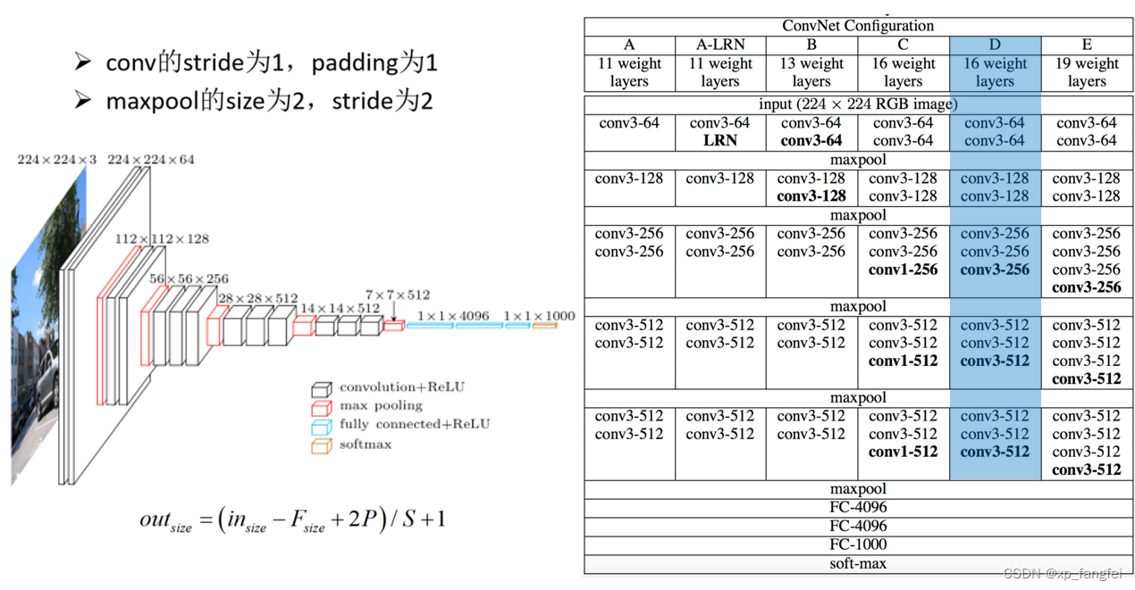
VGG系列模型介绍
- VGG网络有多个版本,一般常用的是VGG-16模型,其网络结构如下如所示:
程序的实现
model.py
mode.py文件主要是模型的实现程序,该模型主要用来进行特征提取。
model.py程序如下:
import torch.nn as nn
import torch
from torchinfo import summary

class VGG(nn.Module):
    def __init__(self, features, num_classes=1000, init_weights=False):
        super(VGG, self).__init__()
        self.features = features			# 卷积层提取特征
        self.classifier = nn.Sequential(	# 全连接层进行分类
            nn.Dropout(p=0.5),
            nn.Linear(512*7*7, 2048),
            nn.ReLU(True),
            nn.Dropout(p=0.5),
            nn.Linear(2048, 2048),
            nn.ReLU(True),
            nn.Linear(2048, num_classes)
        )
        if init_weights:
            self._initialize_weights()

    def forward(self, x):
        # N x 3 x 224 x 224
        x = self.features(x)
        # N x 512 x 7 x 7
        x = torch.flatten(x, start_dim=1)
        # N x 512*7*7
        x = self.classifier(x)
        return x

    def _initialize_weights(self):
        for m in self.modules():
            if isinstance(m, nn.Conv2d):
                # nn.init.kaiming_normal_(m.weight, mode='fan_out', nonlinearity='relu')
                nn.init.xavier_uniform_(m.weight)
                if m.bias is not None:
                    nn.init.constant_(m.bias, 0)
            elif isinstance(m, nn.Linear):
                nn.init.xavier_uniform_(m.weight)
                # nn.init.normal_(m.weight, 0, 0.01)
                nn.init.constant_(m.bias, 0)

# 卷积层提取特征
def make_features(cfg: list):
    layers = []
    in_channels = 3
    for v in cfg:
        if v == "M":
            layers += [nn.MaxPool2d(kernel_size=2, stride=2)]
        else:
            conv2d = nn.Conv2d(in_channels, v, kernel_size=3, padding=1)
            layers += [conv2d, nn.ReLU(True)]
            in_channels = v

    return  nn.Sequential(*layers)               # 单星号(*)将参数以元组的形式导入

def vgg(model_name="vgg16", **kwargs):           # 双星号(**)将参数以字典的形式导入
    try:
        cfg = cfgs[model_name]
    except:
        print("Warning: model number {} not in cfgs dict!".format(model_name))
        exit(-1)
    features = make_features(cfg)
    model = VGG(features, **kwargs)
    return model
VGG几种网络模型参数配置:
# vgg网络模型配置列表,数字表示卷积核个数,'M'表示最大池化层
cfgs = {
    'vgg11': [64, 'M', 128, 'M', 256, 256, 'M', 512, 512, 'M', 512, 512, 'M'],											# 模型A
    'vgg13': [64, 64, 'M', 128, 128, 'M', 256, 256, 'M', 512, 512, 'M', 512, 512, 'M'],									# 模型B
    'vgg16': [64, 64, 'M', 128, 128, 'M', 256, 256, 256, 'M', 512, 512, 512, 'M', 512, 512, 512, 'M'],					# 模型D
    'vgg19': [64, 64, 'M', 128, 128, 'M', 256, 256, 256, 256, 'M', 512, 512, 512, 512, 'M', 512, 512, 512, 512, 'M'], 	# 模型E
}
VGG官方预训练权重下载地址:
# official pretrain weights
model_urls = {
    'vgg11': 'https://download.pytorch.org/models/vgg11-bbd30ac9.pth',
    'vgg13': 'https://download.pytorch.org/models/vgg13-c768596a.pth',
    'vgg16': 'https://download.pytorch.org/models/vgg16-397923af.pth',
    'vgg19': 'https://download.pytorch.org/models/vgg19-dcbb9e9d.pth'
}
train.py
import torch
import torch.nn as nn
from torchvision import transforms, datasets, utils
import matplotlib.pyplot as plt
import numpy as np
import torch.optim as optim
import os

import model
from model import *
from train_tool import TrainTool


#使用GPU训练
device = torch.device("cuda" if torch.cuda.is_available() else "cpu")
print(device)
#数据预处理
transform = {
    "train": transforms.Compose([transforms.Resize((224, 224)),   #随机裁剪,再缩放成224*224
                                 transforms.RandomHorizontalFlip(p=0.5), #水平方向随机翻转,概率为0.5
                                 transforms.ToTensor(),
                                 transforms.Normalize((0.5, 0.5, 0.5),(0.5, 0.5, 0.5))]),
    "test": transforms.Compose([transforms.Resize((224, 224)),
                               transforms.ToTensor(),
                               transforms.Normalize((0.5, 0.5, 0.5),(0.5, 0.5, 0.5))])}
#导入加载数据集
#获取图像数据集的路径
data_root = os.getcwd()
image_path = data_root + "/data_road/"                #根据自己的数据集路径修改
print(image_path)
#导入训练集并进行处理
train_dataset = datasets.ImageFolder(root=image_path + "/train_road",  #根据自己的数据集路径修改
                                     transform=transform["train"])     #和transform中关键字一致
train_num = len(train_dataset)
#加载训练集
train_loader = torch.utils.data.DataLoader(train_dataset,  #导入的训练集
                                           batch_size=8,   #每批训练样本个数
                                           shuffle=True,   #打乱训练集
                                           num_workers=0)  #使用线程数

#导入测试集并进行处理
test_dataset = datasets.ImageFolder(root=image_path + "/test_road",    #根据自己的数据集路径修改
                                     transform=transform["test"])      #和transform中关键字一致
test_num = len(test_dataset)
#加载测试集
test_loader = torch.utils.data.DataLoader(test_dataset,    #导入的测试集
                                           batch_size=8,   #每批测试样本个数
                                           shuffle=True,   #打乱测试集
                                           num_workers=0)  #使用线程数


#定义超参数
model_name = "vgg11"            #根据所使用模型类型进行更改
vgg = model.vgg(model_name=model_name, num_classes=2, init_weights=True).to(device)  # num_classes根据自己情况更改
loss_function = nn.CrossEntropyLoss()  #定义损失函数为交叉熵
optimizer = optim.Adam(vgg.parameters(), lr=0.0002)  #定义优化器定义参数学习率


#正式训练
train_acc = []
train_loss = []
test_acc = []
test_loss = []

epoch = 0

#for epoch in range(epochs):
while True:
    epoch = epoch + 1;
    vgg.train()

    epoch_train_acc, epoch_train_loss = TrainTool.train(train_loader, vgg, optimizer, loss_function, epoch, device)

    vgg.eval()
    epoch_test_acc, epoch_test_loss = TrainTool.test(test_loader,vgg, loss_function, device)
    if epoch_train_acc < 0.99 and epoch_test_acc < 0.99:
       template = ('Epoch:{:2d}, train_acc:{:.1f}%, train_loss:{:.2f}, test_acc:{:.1f}%, test_loss:{:.2f}')
       print(template.format(epoch, epoch_train_acc * 100, epoch_train_loss, epoch_test_acc * 100, epoch_test_loss))
       continue
    else:
       torch.save(vgg.state_dict(),'./model/vgg_params.pth')    #设置训练好模型保存路径
       print('Done')
       break
train_tools.py
import torch
import matplotlib.pyplot as plt

class TrainTool:
      def image_show(images):
          print(images.shape)
          images = images.numpy()   #将图片有tensor转换成array
          print(images.shape)
          images = images.transpose((1, 2, 0))   # 将【3,224,256】-->【224,256,3】
          # std = [0.5, 0.5, 0.5]
          # mean = [0.5, 0.5, 0.5]
          # images = images * std + mean
          print(images.shape)
          plt.imshow(images)
          plt.show()


      def train(train_loader, model, optimizer, loss_function, epoch, device):
          train_size = len(train_loader.dataset)  # 训练集的大小
          num_batches = len(train_loader)  # 批次数目
          train_acc, train_loss = 0, 0  # 初始化正确率和损失

          # 获取图片及标签
          for images, labels in train_loader:
              images, labels = images.to(device), labels.to(device)
              # 计算预测误差
              pred_labels = model(images)
              loss = loss_function(pred_labels, labels)
              # 反向传播
              optimizer.zero_grad()  # grad属性归零
              loss.backward()  # 反向传播
              optimizer.step()  # 每一步自动更新
              # 记录acc和loss
              train_acc += (pred_labels.argmax(1) == labels).type(torch.float).sum().item()
              train_loss += loss.item()

          train_acc /= train_size
          train_loss /= num_batches

          return train_acc, train_loss


      def test(test_loader, model, loss_function, device):
          test_size = len(test_loader.dataset)  # 测试集的大小,一共10000张图片
          num_batches = len(test_loader)  # 批次数目,313(10000/32=312.5,向上取整)
          test_loss, test_acc = 0, 0

          # 当不进行训练时,停止梯度更新,节省计算内存消耗
          with torch.no_grad():
              for images, labels in test_loader:
                  images, labels = images.to(device), labels.to(device)

                  # 计算loss
                  pred_labels = model(images)
                  loss = loss_function(pred_labels, labels)

                  test_acc += (pred_labels.argmax(1) == labels).type(torch.float).sum().item()
                  test_loss += loss.item()

          test_acc /= test_size
          test_loss /= num_batches

          return test_acc, test_loss
predict.py
import torch
import torchvision.transforms as transforms
from PIL import Image
from model import VGG, vgg

#数据预处理
transforms = transforms.Compose([transforms.Resize((224, 224)),
                                 transforms.ToTensor(),
                                 transforms.Normalize((0.5, 0.5, 0.5),(0.5, 0.5, 0.5))])
#导入要测试的图像
image = Image.open('./data_road/val/845.jpg')
image = transforms(image)
image = torch.unsqueeze(image, dim=0)

#实例化网络,加载训练好的模型参数
model_name = "vgg11"
vgg_model = vgg(model_name=model_name, num_classes=2, init_weights=True)  # num_classes根据自己情况更改

vgg_model.load_state_dict(torch.load('./model/vgg_params.pth'))

#预测
classes = ('cross', 'no_cross')        # 根据自己分类情况而定

with torch.no_grad():
    outputs = vgg_model(image)
    print(outputs)
    predict = torch.max(outputs, dim=1)[1].data.numpy()
    print(predict)
print(classes[int(predict)])
如有错误欢迎指正,如果帮到您请点赞加关注谢谢!


 1465
1465


 被折叠的 条评论
为什么被折叠?
被折叠的 条评论
为什么被折叠?
 到【灌水乐园】发言


