图像分类：Pytorch图像分类之-- MobileNet系列模型

xp_fangfei

已于 2023-04-11 09:25:03 修改

阅读量1.2k

点赞数 2

分类专栏：机器学习文章标签： pytorch 分类深度学习

于 2023-04-10 16:37:55 首次发布

本文链接：https://blog.csdn.net/xp_fangfei/article/details/130016297

版权

机器学习专栏收录该内容

25 篇文章 2 订阅

订阅专栏

文章目录

前言

MobileNet网络专注于移动端或者嵌入式设备中的轻量级CNN，相比于传统卷积神经网络，在准确率小幅度降低的前提下大大减少模型参数与运算量。

MobileNetV1模型介绍

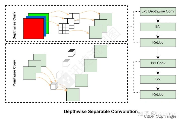
MobileNetV1提出了 Depthwise Separable Convolutions（深度可分离卷积）；深度可分离卷积过程被拆分成了两个部分：深度卷积（Depthwise Convolution）与逐点卷积层（Pointwise Convolution）。

DW（Depthwise Convolution）卷积

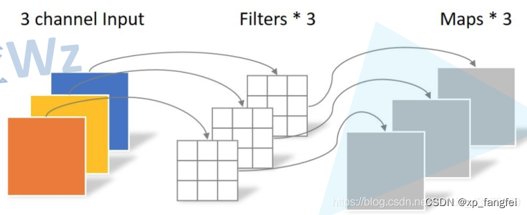
DW卷积中，每个卷积核的channel都为1，每个卷积核只负责与输入特征矩阵中的1个channel进行卷积运算，然后再得到相应的输出特征矩阵中的1个channel。
如下图所示：
在这里插入图片描述

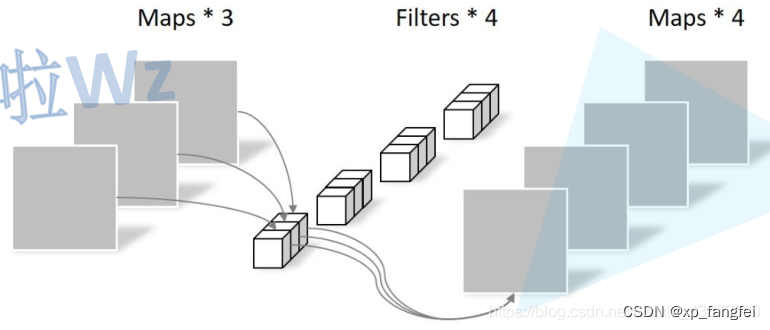
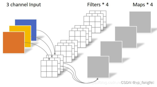
PW （Pointwise Convolution）卷积

PW卷积的特点是卷积核的维度是1*1，从输入到输出可以改变维度，DW和PW通常是一起使用。

深度可分离卷积（DW+PW）

1、深度可分离卷积的计算量
对于深度可分离卷积的DW部分，设输入特征图通道数为M，对特征图进行卷积的核大小为K，则该部分的计算量：
$K * K * M$
对于深度可分离卷积的PW部分，设输出特征图通道数为N，该部分的计算量： $1 * 1 * M * N$
则深度可分离卷积的计算量为：
$K * K * M + 1 * 1 * M * N$

在这里插入图片描述

2、传统卷积的计算量
设输入特征图像的通道为M，输出特征图像的通道为N，对输入特征图像进行卷积的卷积核大小为K，则传统卷积的计算量为： $K * K * M * N$
在这里插入图片描述
3、深度可分离卷积和传统卷积比值
深度可分离卷积的计算量要比传统卷积计算量小，从以下比值可以可以看出：
${深度可分离卷积\over 传统卷积}={K*K*M + 1*1*M*N \over K*K*M*N }= {1\over N }+{1\over K^2 }$

理论上普通卷积计算量是DW+PW的8到9倍。

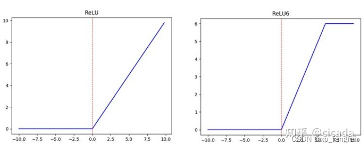
ReLU6激活函数的介绍

ReLU6就是普通的ReLU但是限制最大输出值为6（对输出值做clip），这是为了在移动端设备float16的低精度的时候，也能有很好的数值分辨率，如果对ReLU的激活范围不加限制，输出范围为0到正无穷，如果激活值非常大，分布在一个很大的范围内，则低精度的float16无法很好地精确描述如此大范围的数值，带来精度损失。

如下图所示：
在这里插入图片描述

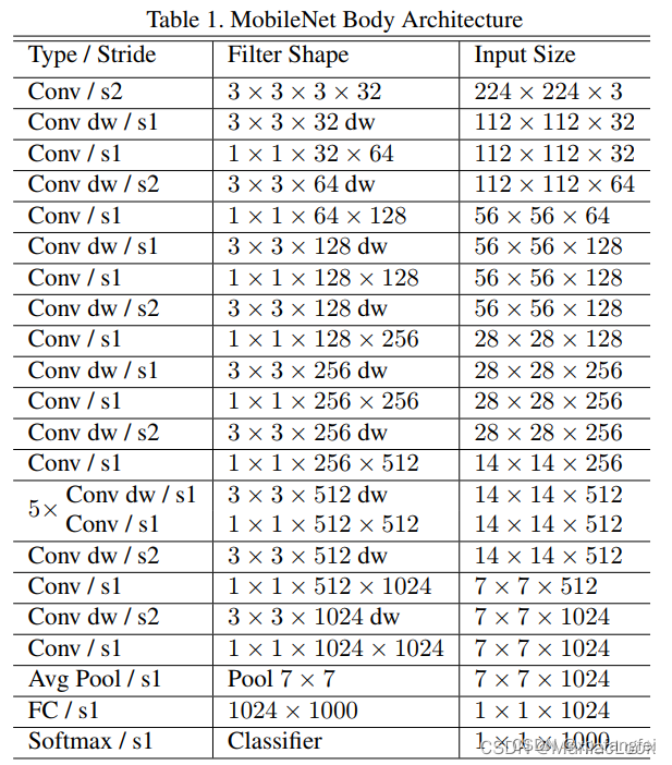
MobileNet V1网络结构

在这里插入图片描述

MobileNet V1程序

import torch
import torch.nn as nn
from torchinfo import summary


def conv_bn(in_channel, out_channel, stride=1):
    """

    传统卷积块：conv + BN + Act
    """
    return nn.Sequential(
        nn.Conv2d(in_channels=in_channel, out_channels=out_channel, kernel_size=3,
                  stride=stride, padding=1, bias=False),
        nn.BatchNorm2d(out_channel),
        nn.ReLU6(inplace=True)
    )


def conv_dsc(in_channel, out_channel, stride=1):
    """

    深度可分离卷积：DW+PW
    """
    return nn.Sequential(
        nn.Conv2d(in_channels=in_channel, out_channels=in_channel,kernel_size=3,
                  stride=stride, padding=1, groups=in_channel, bias=False),
        nn.BatchNorm2d(in_channel),
        nn.ReLU6(inplace=True),


        nn.Conv2d(in_channels=in_channel, out_channels=out_channel, kernel_size=1,
                  stride=1, padding=0, bias=False),
        nn.BatchNorm2d(out_channel),
        nn.ReLU6(inplace=True)

    )
class MobileNetV1(nn.Module):
    def __init__(self, in_channel=3, num_classes=1000):
        super(MobileNetV1, self).__init__()
        self.num_classes = num_classes
        self.stage1 = nn.Sequential(
            conv_bn(in_channel=in_channel, out_channel=32, stride=2),
            conv_dsc(in_channel=32, out_channel=64, stride=1),
            conv_dsc(in_channel=64, out_channel=128, stride=2),
            conv_dsc(in_channel=128, out_channel=128, stride=1),
            conv_dsc(in_channel=128, out_channel=256, stride=2),
            conv_dsc(in_channel=256, out_channel=256, stride=1),
            conv_dsc(in_channel=256, out_channel=512, stride=2)
        )

        self.stage2 = nn.Sequential(
            conv_dsc(in_channel=512, out_channel=512,  stride=1),
            conv_dsc(in_channel=512, out_channel=512, stride=1),
            conv_dsc(in_channel=512, out_channel=512, stride=1),
            conv_dsc(in_channel=512, out_channel=512, stride=1),
            conv_dsc(in_channel=512, out_channel=512, stride=1)
        )

        self.stage3 = nn.Sequential(
            conv_dsc(in_channel=512, out_channel=1024, stride=2),
            conv_dsc(in_channel=1024, out_channel=1024, stride=2)
        )
        self.avg1 = nn.AdaptiveAvgPool2d((1, 1))
        self.fc1 = nn.Linear(1024, num_classes)

    def forward(self, x):
        x = self.stage1(x)
        x = self.stage2(x)
        x = self.stage3(x)
        x = self.avg1(x)
        x = x.view(-1, 1024)
        x = self.fc1(x)

        return x

MobileNetV2模型介绍

MobileNetV2是MobileNet的升级版，它具有一个非常重要的特点就是使用了Inverted resblock，整个mobilenetv2都由Inverted resblock组成。

Inverted residual block介绍

通道越少，卷积层的乘法计算量就越小。那么如果整个网络都是低维的通道，那么整体计算速度就会很快。然而，这样效果并不好，没有办法提取到整体的足够多的信息。所以，如果提取特征数据的话，我们可能更希望有高维的通道来做这个事情。MobileNetV2就设计这样一个结构来达到平衡。
MobileNetV2中首先扩展维度，然后用depthwise conv来提取特征，最后再压缩数据，让网络变小。
在这里插入图片描述
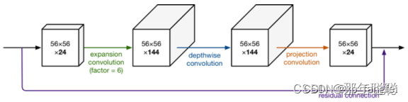
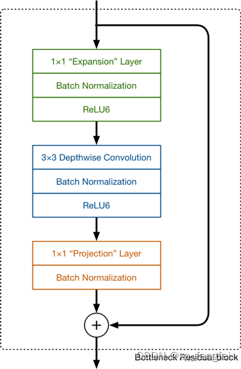
Inverted residual block可以分为两个部分：主要包括Expansion layer，Depthwise Convolution，Projection layer。
Expansion layer表示扩展层，使用1x1卷积，目的是将低维空间映射到高维空间(升维)。
Projection layer表示投影层，使用1x1卷积，目的是把高维特征映射到低维空间去(降维)。
Depthwise Convolution表示深度可分离卷积，完成卷积功能，降低计算量、参数量。

在这里插入图片描述

Inverted residual block 和 residual block的区别

1、结构的不同如下图

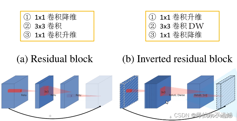
2、激活函数的不同：Inverted residual block中使用的是ReLu6；residual block中使用的是ReLu。

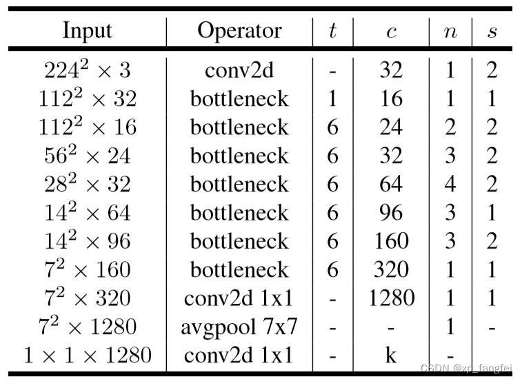
MobileNetV2网络结构

在这里插入图片描述

MobileNetV2程序

import torch
import torch.nn as nn
from torchinfo import summary
import torchvision.models.mobilenetv2
# ------------------------------------------------------#
#   这个函数的目的是确保Channel个数能被8整除。
#	很多嵌入式设备做优化时都采用这个准则
# ------------------------------------------------------#
def _make_divisible(v, divisor, min_value=None):
    if min_value is None:
        min_value = divisor
    new_v = max(min_value, int(v + divisor / 2) // divisor * divisor)
    if new_v < 0.9 * v:
        new_v += divisor
    return new_v

# -------------------------------------------------------------#
#   Conv+BN+ReLU经常会用到，组在一起
#   参数顺序：输入通道数,输出通道数...
#		最后的groups参数：groups=1时，普通卷积；
#						 groups=输入通道数in_planes时，DW卷积=深度可分离卷积
#	pytorch官方继承自nn.sequential，想用它的预训练权重，就得听它的
# -------------------------------------------------------------#
class ConvBNReLU(nn.Sequential):
    def __init__(self, in_planes, out_planes, kernel_size=3, stride=1, groups=1):
        padding = (kernel_size - 1) // 2
        super(ConvBNReLU, self).__init__(
            nn.Conv2d(in_planes, out_planes, kernel_size, stride, padding, groups=groups, bias=False),
            nn.BatchNorm2d(out_planes),
            nn.ReLU6(inplace=True)
        )

# ------------------------------------------------------#
#   InvertedResidual，先升维后降维
#   参数顺序：输入通道数,输出通道数，步长，变胖倍数(扩展因子)
# ------------------------------------------------------#
class InvertedResidual(nn.Module):
    def __init__(self, inp, oup, stride, expand_ratio):
        super(InvertedResidual, self).__init__()
        self.stride = stride
        assert stride in [1, 2]

        hidden_dim = int(round(inp * expand_ratio))
        self.use_res_connect = self.stride == 1 and inp == oup

        layers = []
        if expand_ratio != 1:
            layers.append(ConvBNReLU(inp, hidden_dim, kernel_size=1))
        layers.extend([
            ConvBNReLU(hidden_dim, hidden_dim, stride=stride, groups=hidden_dim),
            nn.Conv2d(hidden_dim, oup, 1, 1, 0, bias=False),
            nn.BatchNorm2d(oup),
        ])
        self.conv = nn.Sequential(*layers)

    def forward(self, x):
        if self.use_res_connect:
            return x + self.conv(x)
        else:
            return self.conv(x)

class MobileNetV2(nn.Module):
    def __init__(self, num_classes=1000, width_mult=1.0, inverted_residual_setting=None, round_nearest=8):
        super(MobileNetV2, self).__init__()
        block = InvertedResidual
        input_channel = 32
        last_channel = 1280

        if inverted_residual_setting is None:
            inverted_residual_setting = [
                # t表示扩展因子(变胖倍数)；c是通道数；n是block重复几次；
                #	s：stride步长，只针对第一层，其它s都等于1
                [1, 16, 1, 1],
                [6, 24, 2, 2],
                [6, 32, 3, 2],
                [6, 64, 4, 2],
                [6, 96, 3, 1],
                [6, 160, 3, 2],
                [6, 320, 1, 1],
            ]

        if len(inverted_residual_setting) == 0 or len(inverted_residual_setting[0]) != 4:
            raise ValueError("inverted_residual_setting should be non-empty "
                             "or a 4-element list, got {}".format(inverted_residual_setting))

        input_channel = _make_divisible(input_channel * width_mult, round_nearest)
        self.last_channel = _make_divisible(last_channel * max(1.0, width_mult), round_nearest)
        features = [ConvBNReLU(3, input_channel, stride=2)]

        for t, c, n, s in inverted_residual_setting:
            output_channel = _make_divisible(c * width_mult, round_nearest)
            for i in range(n):
                stride = s if i == 0 else 1
                features.append(block(input_channel, output_channel, stride, expand_ratio=t))
                input_channel = output_channel

        features.append(ConvBNReLU(input_channel, self.last_channel, kernel_size=1))
        self.features = nn.Sequential(*features)

        self.classifier = nn.Sequential(
            nn.Dropout(0.2),
            nn.Linear(self.last_channel, num_classes),
        )

        for m in self.modules():
            if isinstance(m, nn.Conv2d):
                nn.init.kaiming_normal_(m.weight, mode='fan_out')
                if m.bias is not None:
                    nn.init.zeros_(m.bias)
            elif isinstance(m, nn.BatchNorm2d):
                nn.init.ones_(m.weight)
                nn.init.zeros_(m.bias)
            elif isinstance(m, nn.Linear):
                nn.init.normal_(m.weight, 0, 0.01)
                nn.init.zeros_(m.bias)

    def forward(self, x):
        x = self.features(x)
        x = x.mean([2, 3])
        x = self.classifier(x)
        return x

model = MobileNetV2()
summary(model)

如果有错误欢迎指正，如果帮到您请点赞加收藏哦！

xp_fangfei

关注

2
点赞
踩
5

收藏

觉得还不错? 一键收藏
打赏
0
评论
图像分类：Pytorch图像分类之-- MobileNet系列模型

MobileNet网络专注于移动端或者嵌入式设备中的轻量级CNN，相比于传统卷积神经网络，在准确率小幅度降低的前提下大大减少模型参数与运算量。MobileNetV1提出了 Depthwise Separable Convolutions（深度可分离卷积）；深度可分离卷积过程被拆分成了两个部分：深度卷积（Depthwise Convolution）与逐点卷积层（Pointwise Convolution）。
复制链接

扫一扫