【神经网络】生成对抗网络GAN

生成对抗网络GAN

欢迎访问Blog总目录！

1.学习链接

Generative Adversarial Networks

生成对抗网络（GAN） - 知乎 (zhihu.com)

深度学习----GAN（生成对抗神经网络）原理解析_gan神经网络-CSDN博客

图解 生成对抗网络GAN 原理 超详解_生成对抗网络gan图解-CSDN博客

2.GAN结构

GAN包含两个模型：

• 生成模型（Generator）:接收随机噪声，生成看起来真实的、与原始数据相似的实例。
• 判别模型（Discrimintor）:判断Generator生成的实例是真实的还是人为伪造的。（真实实例来源于数据集，伪造实例来源于生成模型）

最终得到效果极好的生成模型，其生成的实例真假难辨。

GAN的灵感来源于 “零和博弈” （完全竞争博弈），GAN就是通过生成网络G（Generator）和判别网络D（Discriminator）不断博弈，进而使G学习到数据的分布，即达到纳什均衡。

【纳什均衡】博弈中这样的局面，对于每个参与者来说，只要其他人不改变策略，他就无法改善自己的状况。对于GAN，即生成模型 G 恢复了训练数据的分布（造出了和真实数据一模一样的样本），判别模型D判别不出来结果（乱猜），准确率为 50%（收敛）。这样双方网络利益均最大化，不再改变自己的策略（不再更新自己的权重）。

2.1.生成模型Generator

• 输入： 数据集的某些向量信息，此处使用满足常见分布（高斯分布、均值分布等）的随机向量。
• 输出： 符合像素大小的图片。
• 结构： 全连接神经网络或者反卷积网络。

2.2.判别模型Discrimintor

• 输入： 伪造图片和数据集图片
• 输出： 图片的真伪标签
• 结构： 判别器模型（全连接网络、卷积网络等）
  

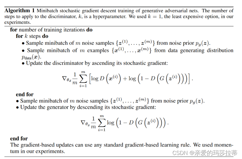
2.3.伪代码

3.优缺点

3.1.优势

• GAN采用的是一种无监督的学习方式训练，可以被广泛用在无监督学习和半监督学习领域
• 模型只用到了反向传播,而不需要马尔科夫链

3.2.缺点

• 难以学习离散数据，如文本

4.pytorch GAN

4.1.API

生成对抗网络 - PyTorch官方教程中文版 (panchuang.net)

4.2.GAN的搭建

绘制在upper_bound和lower_bound之间的一元二次方程画

4.2.1.结果

4.2.2.代码

import torch
import torch.nn as nn
import numpy as np
import matplotlib.pyplot as plt

torch.manual_seed(1)    # reproducible
np.random.seed(1)

# Hyper Parameters
BATCH_SIZE = 64
LR_G = 0.0001           # learning rate for generator
LR_D = 0.0001           # learning rate for discriminator
N_IDEAS = 5             # 噪声点个数
ART_COMPONENTS = 15     # 15个Y轴数据点
PAINT_POINTS = np.vstack([np.linspace(-1, 1, ART_COMPONENTS) for _ in range(BATCH_SIZE)])

# show our beautiful painting range
# plt.plot(PAINT_POINTS[0], 2 * np.power(PAINT_POINTS[0], 2) + 1, c='#74BCFF', lw=3, label='upper bound')
# plt.plot(PAINT_POINTS[0], 1 * np.power(PAINT_POINTS[0], 2) + 0, c='#FF9359', lw=3, label='lower bound')
# plt.legend(loc='upper right')
# plt.show()


def artist_works():     # painting from the famous artist (real target)
    a = np.random.uniform(1, 2, size=BATCH_SIZE)[:, np.newaxis]
    paintings = a * np.power(PAINT_POINTS, 2) + (a-1)
    paintings = torch.from_numpy(paintings).float()
    return paintings

G = nn.Sequential(                      # Generator
    nn.Linear(N_IDEAS, 128),            # random ideas (could from normal distribution)
    nn.ReLU(),
    nn.Linear(128, ART_COMPONENTS),     # making a painting from these random ideas
)

D = nn.Sequential(                      # Discriminator
    nn.Linear(ART_COMPONENTS, 128),     # receive art work either from the famous artist or a newbie like G
    nn.ReLU(),
    nn.Linear(128, 1),
    nn.Sigmoid(),                       # tell the probability that the art work is made by artist
)

opt_D = torch.optim.Adam(D.parameters(), lr=LR_D)
opt_G = torch.optim.Adam(G.parameters(), lr=LR_G)

plt.ion()   # something about continuous plotting

for step in range(10000):
    artist_paintings = artist_works()  # real painting from artist
    G_noise = torch.randn(BATCH_SIZE, N_IDEAS, requires_grad=True)  # random ideas\n
    G_paintings = G(G_noise)                    # fake painting from G (random ideas)
    prob_artist0 = D(artist_paintings)  # 判断真画
    prob_artist1 = D(G_paintings)  # 判断假画

    # D增加真画概率，减少伪画概率; 梯度下降法为减小误差，所以添加-号
    # D_loss越小，prob_artist0越大，prob_artist1越小
    D_loss = - torch.mean(torch.log(prob_artist0) + torch.log(1. - prob_artist1))
    opt_D.zero_grad()
    D_loss.backward(retain_graph=True)  # reusing computational graph
    opt_D.step()


    # 重新采样
    G_noise = torch.randn(BATCH_SIZE, N_IDEAS, requires_grad=True)  # random ideas\n
    G_paintings = G(G_noise)  # fake painting from G (random ideas)
    prob_artist1 = D(G_paintings)  # 判断假画

    # G_loss越小，prob_artist1越大
    G_loss = torch.mean(torch.log(1. - prob_artist1))
    opt_G.zero_grad()
    G_loss.backward()
    opt_G.step()


    if step % 50 == 0:  # plotting
        plt.cla()
        plt.plot(PAINT_POINTS[0], G_paintings.data.numpy()[0], c='#4AD631', lw=3, label='Generated painting', )
        plt.plot(PAINT_POINTS[0], 2 * np.power(PAINT_POINTS[0], 2) + 1, c='#74BCFF', lw=3, label='upper bound')
        plt.plot(PAINT_POINTS[0], 1 * np.power(PAINT_POINTS[0], 2) + 0, c='#FF9359', lw=3, label='lower bound')

        # D 的判断准确度=50%最优
        plt.text(-.5, 2.3, 'D accuracy=%.2f (0.5 for D to converge)' % prob_artist0.data.numpy().mean(),
                 fontdict={'size': 13})

        plt.text(-.5, 2, 'D score= %.2f (-1.38 for G to converge)' % -D_loss.data.numpy(), fontdict={'size': 13})
        plt.ylim((0, 3));
        plt.legend(loc='upper right', fontsize=10);
        plt.draw();
        plt.pause(0.01)

plt.ioff()
plt.show()

4.3.示意图⭐️