Multi-level Optimization (Algeraic & Boolean)

Akimoto Akira

已于 2022-07-01 02:17:53 修改

阅读量1.2k

点赞数 1

分类专栏： Synthesis and Optimization 文章标签：硬件工程算法

于 2021-04-06 01:02:20 首次发布

本文链接：https://blog.csdn.net/zch951127/article/details/115445993

版权

Synthesis and Optimization 专栏收录该内容

8 篇文章

订阅专栏

文章目录

Boolean Logic Network
Algebraic Optimization
- Algebraic basic algorithm used in transformation
- 用来编写filter的理论依据
Boolean Optimization

Multi-level optimization主要的实现方法有两种：一种是Rule-based，另一种是Algorithm-Tansformation。
前者的主要思想是通过和比较Rule中的一些结构范式，查询到网络中可以优化的结构，并用Rule设置的结构在网络中进行替代，最后优化的结果的好坏取决于Rule设计的好坏，直接就可以得到mapping过的网络。这里一章要阐述的则主要是后一种方法，优化分为两个阶段进行：technology independent optimization, technology dependent mapping。前者优化的主要目标是对逻辑表达式进行优化，一般的目标是使表达式中的term(表达式中的项数)或是literal(表达式中的变量)数量最小。而后者的目标是在逻辑表达式已经固定的情况下，将抽象的表达式与实际的元器件进行绑定，使其元器件具有实际的参数例如area和delay，从而使得在实际的设计中得到满足要求的优化结果。

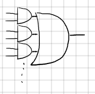
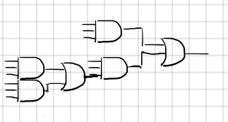
这一章需要阐明的是另一个不同的优化思路 multi-level optimization，这个方法与2-level optimization的区别在于最终结果对逻辑电路的表达方式上。2-level之所以叫做2-level是因为其表达式中只有两层，i.e 表达式的形式为sop (sum of production) 形式"( )+( )+…"，其中()里的一定是一个单项式(monomial或称为term)。而multi-level则会有不止一个层级 i.e ()中可能是一个被使用公因子合并后的多项式，i.e (()()…())+(()()…())()…样式的形式。使用逻辑门来表示则如下Fig1和Fig2所示。

Fig 1. 2-level

Fig 2. multi-level

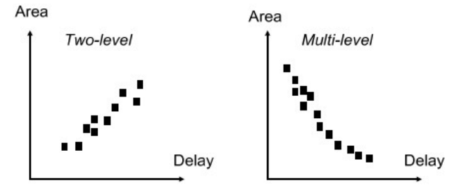
在2-level上其area和delay是兼容的，i.e 当delay减小的时候area也会跟着减小，但是问题在于在这个曲线上能取到的最优点只有一个，即在sop表达方式下的最优解。而在multi-level上可以将所有可能的最优情况考虑进去，从而得到一个parato curve。在这个曲线上所有的点都是一定条件下的最优点，从而可以设定一些限制条件在优化的过程中满足其他参数的要求并且找到满足当前条件的所有最优点。

Fig 3. 2-level & multi-level parato curve

multi-level optimization的实现和heuristic espresso的方法思想很接近，由前面的章节可知，espresso方法通过expand, irredundant和reduce三个算子循环优化得到最优解，而multi-level optimization过程中使用的则是不同的operator，这些operator的核心是对网络中单个节点的transformation，在muti-level optimization中实现方法有两种 Algebraic 和 Boolean。这两种实现方法实际上没有本质的不同，Algebraic transformation 是 Boolean transformation的子集，正是因为Algbraic舍弃了Boolean transformation中的一些操作，虽然说最终的效果没有Boolean这么好，但是其运算速度会更快一些。实际上这个思想在优化算法的优化中经常使用到，为了得到最好的结果，我们可以尝试遍历整个网络中所有的节点，虽然可以得到一个很棒的结果，但是实际操作中会花费很多时间，由其是在网络规模变大后，遍历整个网络花费的时间会更多。因此在优化script中会设置相应的filter来对网络中的优化节点进行过滤，减轻算法的处理负担。

Boolean Logic Network

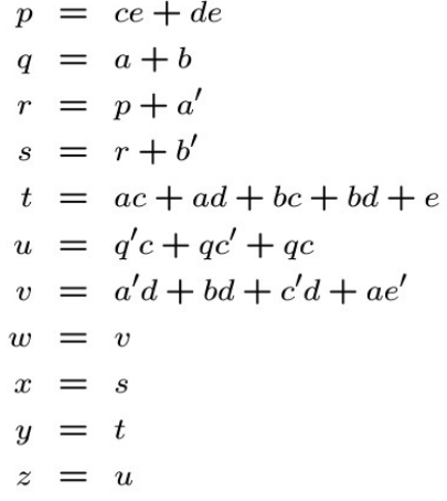
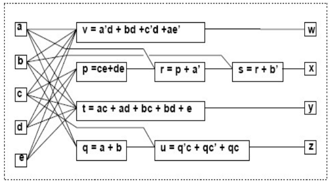
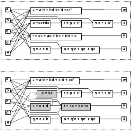
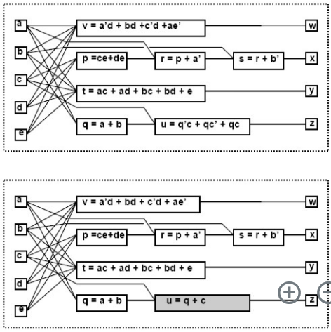
下图是一个boolean logic network的例子，其中的vertices代表了一个逻辑表达式，连接各个vertices的edge代表了各个vertices之间的相互调用之类的关系。图Fig 4中为各个vertices的表达式，Fig 5为boolean logic network模型

Fig 4. vertices definition

Fig 5. boolean logic network wrt vertices in Fig4

Algebraic Optimization

接下来就是对网络的逻辑表达进行优化使其成为parato curve上的一点。在Algebraic实际上做的就是将逻辑表达式看作一个代数表达式来处理，其中互补的代数变量也看作是不同的变量，这样进行因式分解加减等代数操作，而不需要考虑Boolean逻辑运算的法则。基本的Transformation有以下几种：

elimination
消除一个vertex（代换进另一个里）

Fig 6 elimination

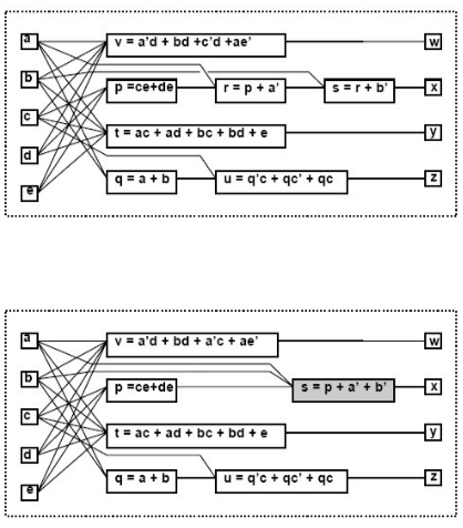
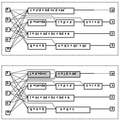
decomposition
将一个vertex展开分为两个

Fig 7 decomposition

substitution
将另一个不在vertex支撑集中的另一个变量代替vertex中的某一部分（会产生新的edge）。简而言之就是用网络中其它的vertex替代另一个vertex中的某些部分，但是在原网络中这样的关系是没有建立的，比如在这里q替代了在t中(a+b)因式。

Fig 8 substitution

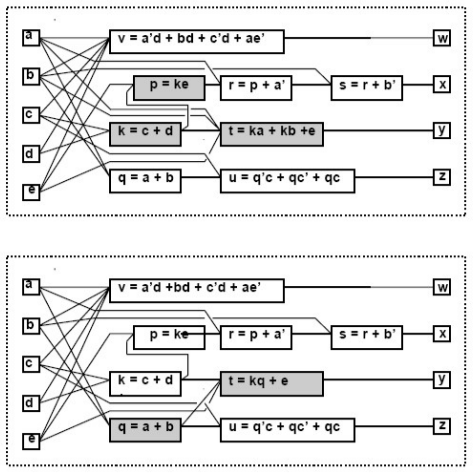
extraction
找出两个节点之间包含的相同的因式提取出来形成一个新的vertex。

Fig9 extraction

simplification
在一个vertex的内部自我优化，使得litera或是term的数量更小。

Fig 10 simplification

由这些transformation我们可以通过添加上一些辅助的代码，使得其成为一个operator。这些辅助代码通常是一些遍历或是filter代码，来帮助transformation可以操作到所有网络中想要优化的部分。通过对这些operator排序可以得到不同的优化结果，这个结果需要程序员慢慢尝试才能针对某一个电路得到比较好的优化结果。

Algebraic basic algorithm used in transformation

Algebraic Division（用于substitution和extraction）
- Predefinition:
  Set-based Notation for Expression：逻辑表达式中的term组成的集合
  Dividend，Divisor，Quotient，Remainder：和普通除法一样的定义
- Algorithm
  
  【注】对于这个D，其实就是一个A中项的集合的子集。在第一个for中遍历的是每一个B的项，在D中则是A中包含for循环选择的项的A的元素。而 $D_{i}$ 则是D去掉项中的B元素。
  e.g $d i v i d e n d = a c + a d + b c + b d + e d i v i s o r = a + b$
  第一次循环中选中B中的项为a。
  D={ac, ad}
  $D_{i}$ ={c,d}
Multiple-Kernel Extraction（用于decomposition）
- Predefinition:
  Cube：因式，不一定是abc这种形式，((abc)d)+e)这样的形式也算是一个cube
  Cube-free expression：不能被因式分解为单个cube的表达式， e.g abc+e, ac+bd等 not cube-free的式子意思就是可以因式分解的, e.g ab+bd等
  Kernel： The cube free quotient of the expression divided by another cube, the divisor, called cokernel
- Algorithm：Recursive Kernel Computation Algorithm

用来编写filter的理论依据

(对于algebraic division快速判断商是否为空) Given algebraic expression $f_{i}$ and $f_{j}$ , then $f_{i} \over f_{j}$ is empty when either:

$f_{j}$ contains a variable not in $f_{i}$
$f_{j}$ contains a term whose support is not contained in that of any term of $f_{i}$
$f_{j}$ contains more terms than $f_{i}$
The count of any variable in $f_{j}$ is higher than in $f_{i}$

(对于kernal extraction的过程快速判断是否有共同的kernel) Two expressions $f_{a}$ and $f_{b}$ have a common multiple-cube divisor $f_{d}$ if and only if

There exist kernels $k_{a} \in K(f_{a})$ and $k_{b} \in K(f_{b})$ such that $f_{d}$ is the sum of two (or more) cubes in $k_{a} \cap k_{b}$ i.e $k_{a}$ 和 $k_{b}$ 的交集元素个数大于或等于2。

Boolean Optimization

DC(Don’t care condition)

在Karnaugh map中会有一些并不在意其取值为1或0的vertices。这些vertices组成的集合称为don’t care set（DC），这些vertices并不会影响到我们最后逻辑电路的取值。所以为了能够获得更加简单的表达式或者进一步优化我们的逻辑电路我们也可以把这一部分给拿进来使用。
如果在外部环境中规定了某一些输入的组合是不会出现的，那么即使是对结果有影响，由于不会出现同样可以看作是don’t care的情况，这样将这些组合集合起来称为external don’t care condition。同样由于逻辑电路自身结构的原因，当截取一部分网络作为对象时，其外部其它网络也会对它产生一些don’t care condition，这一部分由网络结构产生的DC称为internal don’t care condition。

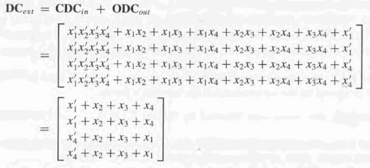
external DC 主要包含了两个部分。一部分是ODC(output observability don’t care sets)这一部分是由于某些原因无法在输出端观测到结果的patterns，另一部分是 CDC(input controllability don’t care sets)，这一部分是在环境中无法产生的一部分输入pattern。我们可以得出以下的关系：
$DC_{extern}=CDC_{in} \cup ODC_{out}$
【注】这个关系是针对一个网络对象而言的，这个网络也可以是一个网络中的子网络。用于探究其它结构对这个子网络的影响也是可以的。

用线性代数的方式来表达这个关系如图Fig11所示。其中的第一列就是CDCin部分，剩下的三列就是ODCout部分。

Fig 11 DC

目前的结构如下图所示，使用前一个网络输出端口的CDC和后一个网络回传的ODC来优化当前网络：
在这里插入图片描述

Satisfiable Don’t Care

一个网络可以看作是多个子网络组成的长链，从而对于此我们可以理解为后一个网络的输入为前一个网络的输出结果。satisfiability don’t care 则是前一个网络DC condition给后一个网络的输出，即可以作为后一个网络计算的起点。
$SDC_{x}=\sum_{all\ internal\ nodes} x \oplus f_{x}$
这个式子的意义是计算出x与自身表达式计算结果不同的部分。后一个网络的化简即可以用 $y+SDC_{x}$ 的来处理。
【注】一个很重要的思想，在SDC或者是 $CDC_{ext}$ 中因为我们并不要关心其表达式结果到底为1或0，因此其所有其中包含的项都可以自己定义其是取1还是取0。因此多余的不拿来优化的项值我们可以取0。这样就不会改变网络本身的值，又可以简化网络。

Output CDC Computation

令输入为 $CDC_{in}$ 。如果没有CDC输入的话 $CDC_{in}=CDC_{ext}=\empty$ (这样算出来就是网络自身的 $CDC_{int}$ )。算法如Fig12所示

在这里插入图片描述

Fig12 CDC calculation

e.g 计算Fig13中的 $CDC_{out}$

在这里插入图片描述

Fig13
初始时C为所有的输入节点 i.e

C=\left \{ x_{1}, x_{2}, x_{3}, x_{4} \right \}

；

CDC_{cut}=CDC_{in}

对于a节点有：

C_{a}=C\cup a=\left \{ x_{1}, x_{2}, x_{3}, x_{4}, a\right \}

CDC_{cut}=CDC_{cut}+a \oplus f_{a}=CDC_{cut}+a \oplus (x_{2} \oplus x_{3})

由于此时添加了a，因此在CDC中需要将

x_{2}, x_{3}

去掉，这里使用concensus操作
i.e

CDC_{cut}=CDC_{cut}|_{x_{2}} \cdot CDC_{cut}|_{x_{2}'}

CDC_{cut}=CDC_{cut}|_{x_{3}} \cdot CDC_{cut}|_{x_{3}'}

然后再在C中将

x_{2}

和

x_{3}

删掉

C=\left \{ x_{1}, x_{4}, a\right \}

…(一个一个逻辑门计算，分别循环传递到

z_{1}

和

z_{2}

)
【注】然后在此网络之后就可以拿这两个输出端口的

C D C

作为后面网络的

CDC_{in}

进行逻辑优化。

Input ODC Computation

这个和前一个相反，由 $ODC_{out}$ 从输出往前推导。推导公式如下：
$ODC_{x}=ODC_{out}+(\frac {\partial f} {\partial x})$
其中f为网络的表达式，x为网络的输入端口。
【注】上面的方法只适用于tree like network，当遇到有多个网络共用同一个输入的情况，在端口上的ODC是多个网络传递的ODC的叠加。