《Keras 3 使用 Swin Transformers 进行图像分类》：此文为AI自动翻译

Keras 3 使用 Swin Transformers 进行图像分类

作者：Rishit Dagli
创建日期：2021/09/08
最后修改时间：2021/09/08
描述：使用 Swin Transformers（计算机视觉的通用主干）进行图像分类。

（i） 此示例使用 Keras 3

 在 Colab 中查看 

 GitHub 源

此示例实现了 Swin Transformer：使用 Shifted Windows 的 Swin Transformer for image classification，并在 CIFAR-100 数据集上进行了演示。

Swin Transformer （Shifted Window Transformer） 可用作 用于计算机视觉的通用主干。Swin Transformer 是一个分层的 Transformer 的表示是通过移位窗口计算的。这 Shifted Window 方案通过限制自我注意带来更高的效率 计算到不重叠的本地窗口，同时还允许 跨窗口连接。此体系结构具有建模的灵活性 信息，并且具有线性计算复杂度，并且 关于图像大小。

此示例需要 TensorFlow 2.5 或更高版本。

---

设置

import matplotlib.pyplot as plt
import numpy as np
import tensorflow as tf  # For tf.data and preprocessing only.
import keras
from keras import layers
from keras import ops

---

配置超参数

要拾取的关键参数是 ，即输入 Patch 的大小。 要将每个像素用作单独的输入，您可以设置为 。下面，我们从原始的纸张设置中汲取灵感 在 ImageNet-1K 上进行训练，保留此示例的大部分原始设置。patch_sizepatch_size(1, 1)

num_classes = 100
input_shape = (32, 32, 3)

patch_size = (2, 2)  # 2-by-2 sized patches
dropout_rate = 0.03  # Dropout rate
num_heads = 8  # Attention heads
embed_dim = 64  # Embedding dimension
num_mlp = 256  # MLP layer size
# Convert embedded patches to query, key, and values with a learnable additive
# value
qkv_bias = True
window_size = 2  # Size of attention window
shift_size = 1  # Size of shifting window
image_dimension = 32  # Initial image size

num_patch_x = input_shape[0] // patch_size[0]
num_patch_y = input_shape[1] // patch_size[1]

learning_rate = 1e-3
batch_size = 128
num_epochs = 40
validation_split = 0.1
weight_decay = 0.0001
label_smoothing = 0.1

---

准备数据

我们通过 加载 CIFAR-100 数据集 。 对图像进行归一化，并将整数标签转换为 one-hot 编码向量。keras.datasets

(x_train, y_train), (x_test, y_test) = keras.datasets.cifar100.load_data()
x_train, x_test = x_train / 255.0, x_test / 255.0
y_train = keras.utils.to_categorical(y_train, num_classes)
y_test = keras.utils.to_categorical(y_test, num_classes)
num_train_samples = int(len(x_train) * (1 - validation_split))
num_val_samples = len(x_train) - num_train_samples
x_train, x_val = np.split(x_train, [num_train_samples])
y_train, y_val = np.split(y_train, [num_train_samples])
print(f"x_train shape: {
       
       x_train.shape} - y_train shape: {
       
       y_train.shape}")
print(f"x_test shape: {
       
       x_test.shape} - y_test shape: {
       
       y_test.shape}")

plt.figure(figsize=(10, 10))
for i in range(25):
    plt.subplot(5, 5, i + 1)
    plt.xticks([])
    plt.yticks([])
    plt.grid(False)
    plt.imshow(x_train[i])
plt.show()

x_train shape: (45000, 32, 32, 3) - y_train shape: (45000, 100) x_test shape: (10000, 32, 32, 3) - y_test shape: (10000, 100)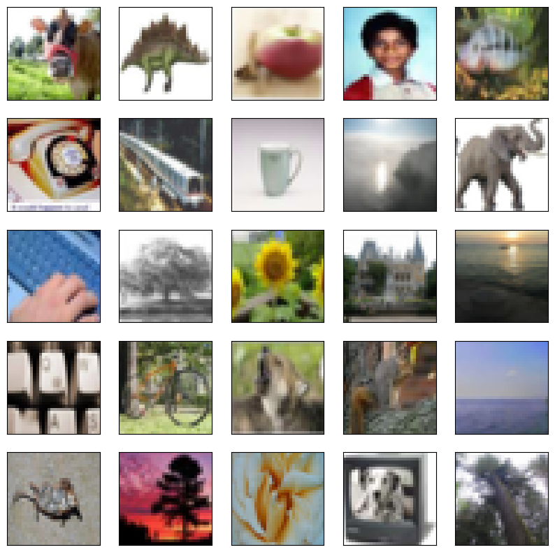 

---

帮助程序函数

我们创建两个辅助函数来帮助我们获取 映像中的修补程序、合并修补程序和应用丢弃。

def window_partition(x, window_size):
    _, height, width, channels = x.shape
    patch_num_y = height // window_size
    patch_num_x = width // window_size
    x = ops.reshape(
        x,
        (
            -1,
            patch_num_y,
            window_size,
            patch_num_x,
            window_size,
            channels,
        ),
    )
    x = ops.transpose(x, (0, 1, 3, 2, 4, 5))
    windows = ops.reshape(x, (-1, window_size, window_size, channels))
    return windows


def window_reverse(windows, window_size, height, width, channels):
    patch_num_y = height // window_size
    patch_num_x = width // window_size
    x = ops.reshape(
        windows,
        (
            -1,
            patch_num_y,
            patch_num_x,
            window_size,
            window_size,
            channels,
        ),
    )
    x = ops.transpose(x, (0, 1, 3, 2, 4, 5))
    x = ops.reshape(x, (-1, height, width, channels))
    return x

---

基于窗口的多头自注意力

通常 Transformer 执行全局自注意，其中关系 计算令牌和所有其他令牌之间的值。全球计算领先 到标记数量的二次复杂度。在这里，正如原始论文所建议的那样，我们计算 在本地窗口中以非重叠的方式进行自我关注。全球 自我注意导致 补丁，而基于窗口的自我注意会导致线性复杂性，并且 易于扩展。

class WindowAttention(layers.Layer):
    def __init__(
        self,
        dim,
        window_size,
        num_heads,
        qkv_bias=True,
        dropout_rate=0.0,
        **kwargs,
    ):
        super().__init__(**kwargs)
        self.dim = dim
        self.window_size =