P7周:基于pytorch的咖啡豆识别-(VGG16复现)

zoey123456789

已于 2024-06-05 15:19:17 修改

阅读量945

点赞数 7

文章标签： pytorch python

于 2024-06-05 08:03:40 首次发布

本文链接：https://blog.csdn.net/zoey123456789/article/details/139457948

版权

第P7周：咖啡豆识别（VGG-16复现）

🍨 本文为🔗365天深度学习训练营中的学习记录博客
🍖 原作者：K同学啊

🍺要求：

自己搭建VGG-16网络框架
调用官方的VGG-16网络框架
如何查看模型的参数量以及相关指标

🍻拔高（可选）：

验证集准确率达到100%
使用PPT画出VGG-16算法框架图（发论文需要这项技能）

🔎探索（难度有点大）

在不影响准确率的前提下轻量化模型

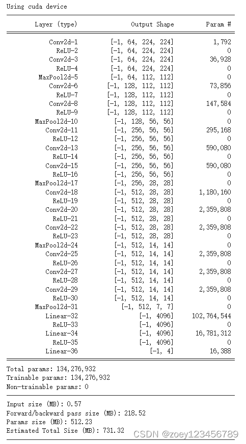
目前VGG16的Total params是134,276,932

我的环境：

语言：python 3.10.12
编译器：Google Colab
深度学习环境：PyTorch
torch == 2.3.0+cu121
torchvision == 0.18.0+cu121

一、前期准备

1.设置GPU（无则用CPU）

import torch
import torch.nn as nn
import torchvision.transforms as transforms
import torchvision
from torchvision import transforms, datasets
import os,PIL,pathlib,warnings

warnings.filterwarnings("ignore")             #忽略警告信息

device = torch.device("cuda" if torch.cuda.is_available() else "cpu")
device

device(type='cuda')

2.导入数据

from google.colab import drive
drive.mount("/content/drive/")

Mounted at /content/drive/

%cd "/content/drive/MyDrive/Colab Notebooks/jupyter notebook/data"

/content/drive/Othercomputers/My laptop/jupyter notebook/data

data_dir = './P7/'
data_dir = pathlib.Path(data_dir)

data_paths  = list(data_dir.glob('*'))
ClassNames = [str(path).split("/")[1] for path in data_paths]
ClassNames

['Dark', 'Green', 'Light', 'Medium']

# 关于transforms.Compose的更多介绍可以参考：https://blog.csdn.net/qq_38251616/article/details/124878863
train_transforms = transforms.Compose([
    transforms.Resize([224, 224]),  # 将输入图片resize成统一尺寸
    #transforms.RandomHorizontalFlip(), # 随机水平翻转
    transforms.ToTensor(), # 将PIL Image或numpy.ndarray转换为tensor，并归一化到[0,1]之间
    transforms.Normalize(     # 标准化处理-->转换为标准正太分布（高斯分布），使模型更容易收敛
    mean=[0.485, 0.456, 0.406],
    std=[0.229, 0.224, 0.225])  # 其中 mean=[0.485,0.456,0.406]与std=[0.229,0.224,0.225] 从数据集中随机抽样计算得到的。
])

test_transforms = transforms.Compose([
  transforms.Resize([224, 224]),  # 将输入图片resize成统一尺寸
   #transforms.RandomHorizontalFlip(), # 随机水平翻转
    transforms.ToTensor(), # 将PIL Image或numpy.ndarray转换为tensor，并归一化到[0,1]之间
    transforms.Normalize(     # 标准化处理-->转换为标准正太分布（高斯分布），使模型更容易收敛
    mean=[0.485, 0.456, 0.406],
    std=[0.229, 0.224, 0.225])  # 其中 mean=[0.485,0.456,0.406]与std=[0.229,0.224,0.225] 从数据集中随机抽样计算得到的。
])

total_data = datasets.ImageFolder("./P7/",transform = train_transforms)
total_data

Dataset ImageFolder
        Number of datapoints: 1200
        Root location: ./P7/
        StandardTransform
    Transform: Compose(
                   Resize(size=[224, 224], interpolation=bilinear, max_size=None, antialias=True)
                   ToTensor()
                   Normalize(mean=[0.485, 0.456, 0.406], std=[0.229, 0.224, 0.225])
               )

total_data.class_to_idx

{'Dark': 0, 'Green': 1, 'Light': 2, 'Medium': 3}

3.划分数据集

train_size = int(0.8 * len(total_data))
test_size  = len(total_data) - train_size
train_dataset, test_dataset = torch.utils.data.random_split(total_data, [train_size, test_size])
train_dataset, test_dataset

(<torch.utils.data.dataset.Subset at 0x7c1bc3e465f0>,
<torch.utils.data.dataset.Subset at 0x7c1bc3e47b50>)

batch_size = 32

train_dl = torch.utils.data.DataLoader(train_dataset, batch_size=batch_size,
                     shuffle = True, num_workers = 1)
test_dl = torch.utils.data.DataLoader(test_dataset, batch_size=batch_size,
                    shuffle = True, num_workers = 1)

for X, y in test_dl:
  print("shape of X [N,C,H,W]:",X.shape)
  print("shape of y:",y.shape,y.dtype)
  break

shape of X [N,C,H,W]: torch.Size([32, 3, 224, 224])
shape of y: torch.Size([32]) torch.int64

二、手动搭建VGG-16

在这里插入图片描述

VGG-16（Visual Geometry Group-16）是由牛津大学视觉几何组（Visual Geometry Group）提出的一种深度卷积神经网络架构，用于图像分类和对象识别任务。VGG-16在2014年被提出，是VGG系列中的一种。VGG-16之所以备受关注，是因为它在ImageNet图像识别竞赛中取得了很好的成绩，展示了其在大规模图像识别任务中的有效性。

以下是VGG-16的主要特点：

深度：VGG-16由16个卷积层和3个全连接层组成，因此具有相对较深的网络结构。这种深度有助于网络学习到更加抽象和复杂的特征。
卷积层的设计：VGG-16的卷积层全部采用3x3的卷积核和步长为1的卷积操作，同时在卷积层之后都接有ReLU激活函数。这种设计的好处在于，通过堆叠多个较小的卷积核，可以提高网络的非线性建模能力，同时减少了参数数量，从而降低了过拟合的风险。
池化层：在卷积层之后，VGG-16使用最大池化层来减少特征图的空间尺寸，帮助提取更加显著的特征并减少计算量。
全连接层：VGG-16在卷积层之后接有3个全连接层，最后一个全连接层输出与类别数相对应的向量，用于进行分类。

VGG-16结构说明：

13个卷积层：分别用blockX_convX表示
3个全连接层：用classifier表示
5个池化层

1.搭建模型

import torch.nn.functional as F

class vgg16(nn.Module):
  def __init__(self):
    super(vgg16, self).__init__()
    # 卷积块1
    self.block1 = nn.Sequential(
        nn.Conv2d(3, 64, kernel_size=(3, 3), stride=(1, 1), padding=(1, 1)),
        nn.ReLU(),
        nn.Conv2d(64, 64, kernel_size=(3, 3), stride=(1, 1), padding=(1, 1)),
        #nn.BatchNorm2d(64),
        nn.ReLU(),
        nn.MaxPool2d(kernel_size=(2, 2), stride=(2, 2))

    )
    # 卷积块2
    self.block2 = nn.Sequential(
        nn.Conv2d(64, 128, kernel_size=(3, 3), stride=(1, 1), padding=(1, 1)),
        nn.ReLU(),
        nn.Conv2d(128, 128, kernel_size=(3, 3), stride=(1, 1), padding=(1, 1)),
        nn.ReLU(),
        #nn.BatchNorm2d(128),
        nn.MaxPool2d(kernel_size=(2,2), stride=(2, 2))
        )
    # 卷积块3
    self.block3 = nn.Sequential(
        nn.Conv2d(128, 256, kernel_size=(3, 3), stride=(1, 1), padding=(1, 1)),
        nn.ReLU(),
        nn.Conv2d(256, 256, kernel_size=(3, 3), stride=(1, 1), padding=(1, 1)),
        nn.ReLU(),
        nn.Conv2d(256, 256, kernel_size=(3, 3), stride=(1, 1), padding=(1, 1)),
        nn.ReLU(),
        #nn.BatchNorm2d(256),
        nn.MaxPool2d(kernel_size=(2, 2), stride=(2, 2))
    )
        # 卷积块4
    self.block4 = nn.Sequential(
        nn.Conv2d(256, 512, kernel_size=(3, 3), stride=(1, 1), padding=(1, 1)),
        nn.ReLU(),
        nn.Conv2d(512, 512, kernel_size=(3, 3), stride=(1, 1), padding=(1, 1)),
        nn.ReLU(),
        nn.Conv2d(512, 512, kernel_size=(3, 3), stride=(1, 1), padding=(1, 1)),
        nn.ReLU(),
        #nn.BatchNorm2d(512),
        nn.MaxPool2d(kernel_size=(2, 2), stride=(2, 2))
    )
        # 卷积块5
    self.block5 = nn.Sequential(
        nn.Conv2d(512, 512, kernel_size=(3, 3), stride=(1, 1), padding=(1, 1)),
        nn.ReLU(),
        nn.Conv2d(512, 512, kernel_size=(3, 3), stride=(1, 1), padding=(1, 1)),
        nn.ReLU(),
        nn.Conv2d(512, 512, kernel_size=(3, 3), stride=(1, 1), padding=(1, 1)),
        nn.ReLU(),
        #nn.BatchNorm2d(512),
        nn.MaxPool2d(kernel_size=(2, 2), stride=(2, 2))
        )

        # 全连接网络层，用于分类
    self.classifier = nn.Sequential(
        nn.Linear(in_features=512*7*7, out_features=4096),
        nn.ReLU(),
        nn.Linear(in_features=4096, out_features=4096),
        nn.ReLU(),
        nn.Linear(in_features=4096, out_features=4)
        )

  def forward(self, x):
    x = self.block1(x)
    x = self.block2(x)
    x = self.block3(x)
    x = self.block4(x)
    x = self.block5(x)
    x = torch.flatten(x, start_dim=1)
    x = self.classifier(x)

    return x

#  def _initialize_weights(self):
#    for m in self.modules():
#      if isinstance(m, nn.Conv2d):
#        nn.init.kaiming_normal_(m.weight, mode='fan_out', nonlinearity='relu')
#        if m.bias is not None:
#          nn.init.constant_(m.bias, 0)
#      elif isinstance(m, nn.Linear):
 #       nn.init.normal_(m.weight, 0, 0.01)
 #       nn.init.constant_(m.bias, 0)


device = "cuda" if torch.cuda.is_available() else "cpu"
print("Using {} device".format(device))

model = vgg16().to(device)

import torchsummary as summary
summary.summary(model,(3,224,224))

在这里插入图片描述

三、训练模型

1.编写训练函数

# 训练循环
def train(dataloader, model, loss_fn, optimizer):
    size = len(dataloader.dataset)  # 训练集的大小
    num_batches = len(dataloader)   # 批次数目, (size/batch_size，向上取整)

    train_loss, train_acc = 0, 0  # 初始化训练损失和正确率

    for X, y in dataloader:  # 获取图片及其标签
        X, y = X.to(device), y.to(device)

        # 计算预测误差
        pred = model(X)          # 网络输出
        loss = loss_fn(pred, y)  # 计算网络输出和真实值之间的差距，targets为真实值，计算二者差值即为损失

        # 反向传播
        optimizer.zero_grad()  # grad属性归零
        loss.backward()        # 反向传播
        optimizer.step()       # 每一步自动更新

        # 记录acc与loss
        train_acc  += (pred.argmax(1) == y).type(torch.float).sum().item()
        train_loss += loss.item()

    train_acc  /= size
    train_loss /= num_batches

    return train_acc, train_loss

2.编写测试函数

def test (dataloader, model, loss_fn):
    size  = len(dataloader.dataset)  # 测试集的大小
    num_batches = len(dataloader) # 批次数目, (size/batch_size，向上取整)
    test_loss, test_acc = 0, 0

    # 当不进行训练时，停止梯度更新，节省计算内存消耗
    with torch.no_grad():
        for imgs, target in dataloader:
            imgs, target = imgs.to(device), target.to(device)

            # 计算loss
            target_pred = model(imgs)
            loss = loss_fn(target_pred, target)

            test_loss += loss.item()
            test_acc  += (target_pred.argmax(1) == target).type(torch.float).sum().item()

    test_acc  /= size
    test_loss /= num_batches

    return test_acc, test_loss

3.学习率设置

# def adjust_learning_rate(optimizer, epoch, start_lr):
# 每 2 个epoch衰减到原来的 0.98
# lr = start_lr * (0.92 ** (epoch // 2))
# for param_group in optimizer.param_groups:
# param_group['lr'] = lr

learn_rate = 1e-4 # 初始学习率
# optimizer  = torch.optim.SGD(model.parameters(), lr=learn_rate)

# 调用官方动态学习率接口时使用
#lambda1 = lambda epoch: 0.92 ** (epoch // 4)
optimizer = torch.optim.Adam(model.parameters(), lr=learn_rate)
#scheduler = torch.optim.lr_scheduler.LambdaLR(optimizer, lr_lambda=lambda1) #选定调整方法

更多的官方动态学习率设置方式可参考：https://pytorch.org/docs/stable/optim.html

4.正式训练

model.train()、model.eval()训练营往期文章中有详细的介绍。

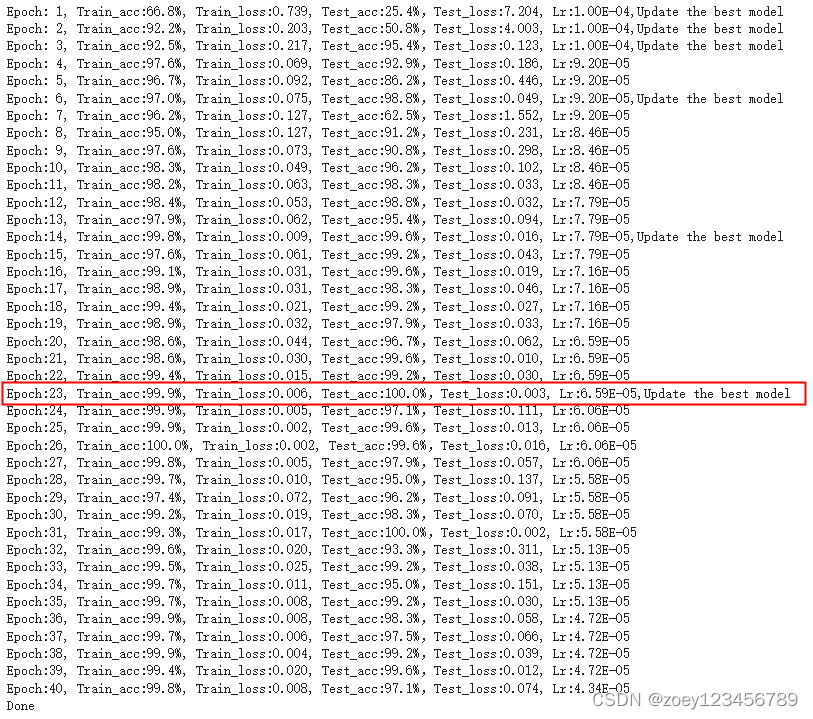
如果将Adam优化器换成SGD会出现40个epoch内准确率和loss都一直不变（不收敛），尝试在每个block中引入batchnorm并修改了初始学习率（并用动态学习率）可以解决该问题，在这过程中加快了模型收敛（如下）。
在这里插入图片描述

SGD的优点是实现简单，计算效率高。但是缺点是可能会陷入局部最优，而且对所有参数使用相同的学习率，如果数据稀疏或者特征尺度差别大，可能导致训练效果不佳。

Adam的优点是结合了RMSProp和Momentum的优点，既考虑了历史梯度的方向，又考虑了当前梯度的大小，因此能够适应性地调整学习率，而且对参数的初始值和学习率的选择不敏感。但是缺点是需要存储每个参数的一阶矩估计和二阶矩估计，所以空间复杂度较高。

具体机制方面，SGD每次只使用一个样本的梯度来更新权重，而Adam则是在SGD的基础上加入了动量和RMSProp。动量可以帮助优化器在相关方向上加速，避免在无关方向上震荡；RMSProp则是通过调整学习率来加快收敛速度。

import copy

optimizer  = torch.optim.Adam(model.parameters(), lr= 1e-4)
loss_fn  = nn.CrossEntropyLoss() # 创建损失函数
epochs   = 40

train_loss = []
train_acc  = []
test_loss  = []
test_acc   = []

best_acc = 0   # 设置一个最佳准确率，作为最佳模型的判别指标

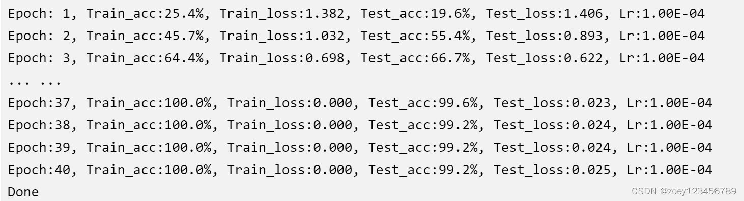
for epoch in range(epochs):
    # 更新学习率（使用自定义学习率时使用）
    # adjust_learning_rate(optimizer, epoch, learn_rate)

    model.train()
    epoch_train_acc, epoch_train_loss = train(train_dl, model, loss_fn, optimizer)
    # scheduler.step() # 更新学习率（调用官方动态学习率接口时使用）

    model.eval()
    epoch_test_acc, epoch_test_loss = test(test_dl, model, loss_fn)

    # 保存最佳模型到 best_model
    if epoch_test_acc > best_acc:
      best_acc  = epoch_test_acc
      best_model = copy.deepcopy(model)

    train_acc.append(epoch_train_acc)
    train_loss.append(epoch_train_loss)
    test_acc.append(epoch_test_acc)
    test_loss.append(epoch_test_loss)

    # 获取当前的学习率
    lr = optimizer.state_dict()['param_groups'][0]['lr']

    template = ('Epoch:{:2d}, Train_acc:{:.1f}%, Train_loss:{:.3f}, Test_acc:{:.1f}%, Test_loss:{:.3f}, Lr:{:.2E}')
    print(template.format(epoch+1, epoch_train_acc*100, epoch_train_loss, epoch_test_acc*100, epoch_test_loss, lr))

# 保存最佳模型到文件中
PATH ='./best_model.pth' # 保存的参数文件名
torch.save(model.state_dict(), PATH)

print('Done')

在这里插入图片描述

四、结果可视化

1.Loss与Accuracy图

import matplotlib.pyplot as plt
#隐藏警告
import warnings
warnings.filterwarnings("ignore")  #忽略警告信息

plt.rcParams['axes.unicode_minus'] = False  # 用来正常显示负号
plt.rcParams['figure.dpi'] = 100        #分辨率

epochs_range = range(epochs)

plt.figure(figsize=(12, 3))
plt.subplot(1, 2, 1)

plt.plot(epochs_range, train_acc, label='Training Accuracy')
plt.plot(epochs_range, test_acc, label='Test Accuracy')
plt.legend(loc='lower right')
plt.title('Training and Validation Accuracy')

plt.subplot(1, 2, 2)
plt.plot(epochs_range, train_loss, label='Training Loss')
plt.plot(epochs_range, test_loss, label='Test Loss')
plt.legend(loc='upper right')
plt.title('Training and Validation Loss')
plt.show()

在这里插入图片描述

2.指定图片进行预测

from PIL import Image

classes = list(total_data.class_to_idx)

def predict_one_image(image_path, model, transform, classes):
  test_img = Image.open(image_path).convert('RGB')
  plt.imshow(test_img)  # 展示预测的图片

  test_img = transform(test_img)
  img = test_img.to(device).unsqueeze(0)

  model.eval()
  output = model(img)

  _,pred = torch.max(output,1)
  pred_class = classes[pred]
  print(f'预测结果是：{pred_class}')

# 预测训练集中的某张照片
predict_one_image(image_path='./P7/Medium/medium (193).png',
                  model=model,
                  transform=train_transforms,
                  classes=classes)

预测结果是：Medium

在这里插入图片描述

3.模型评估

best_model.eval()
epoch_test_acc, epoch_test_loss = test(test_dl, best_model, loss_fn)

epoch_test_acc, epoch_test_loss

在这里插入图片描述

# 查看是否与我们记录的最高准确率一致
epoch_test_acc

0.9958333333333333

五、其他尝试

1.调用官方模型训练

from torchvision.models import vgg16

# 加载预训练模型，并且对模型进行微调
model = vgg16(pretrained = True).to(device) # 加载预训练的vgg16模型

for param in model.parameters():
  param.requires_grad = False # 冻结模型的参数，这样子在训练的时候只训练最后一层的参数

# 修改classifier模块的第6层（即：(6): Linear(in_features=4096, out_features=2, bias=True)）
# 注意查看我们下方打印出来的模型
model.classifier._modules['6'] = nn.Linear(4096,len(ClassNames)) # 修改vgg16模型中最后一层全连接层，输出目标类别个数
model.to(device)
import torchsummary as summary
summary.summary(model,(3,224,224))

在这里插入图片描述

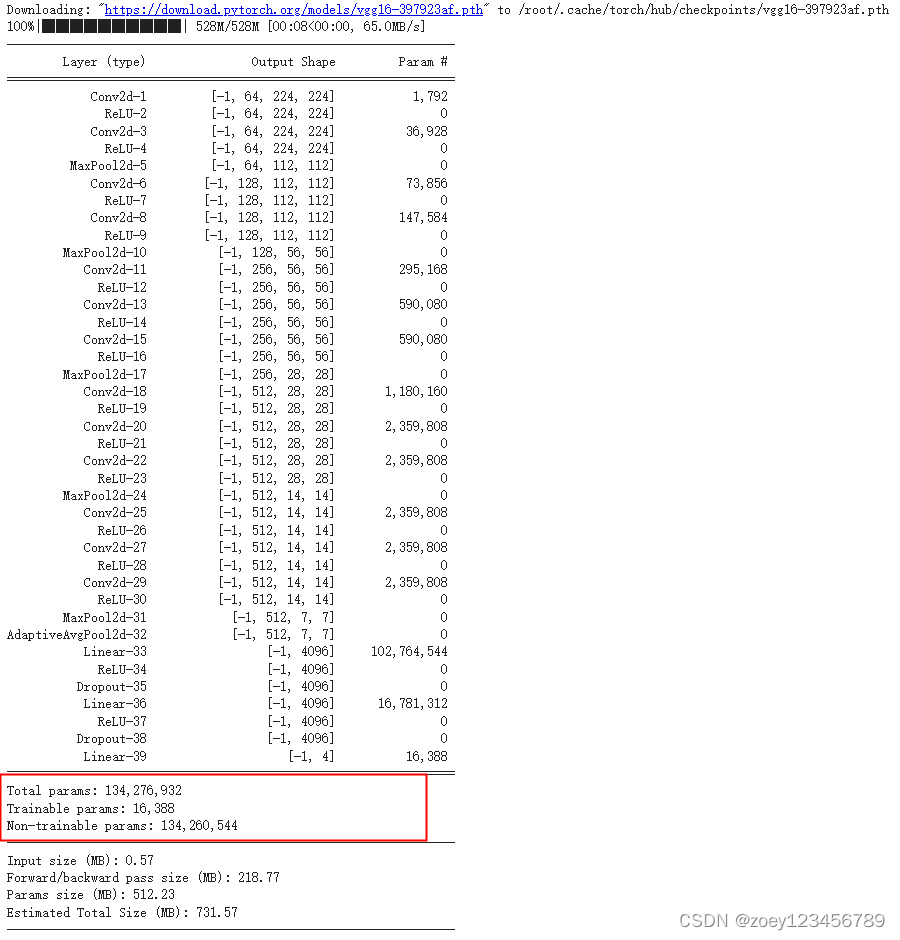
其余条件都不改变，训练结果如下：test acc不如前文手动搭建结果
在这里插入图片描述

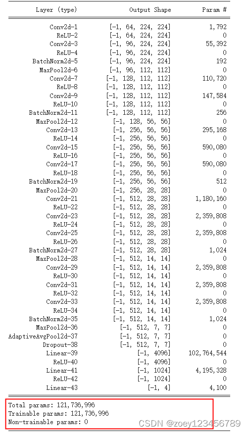
2.轻量化vgg16+提高test acc

基于手动搭建的vgg模型修改，具体如下：

对训练集图像进行随机水平翻转
修改了block1和2中的部分卷积层参数
在每个卷积块中的最大池化之前使用批量归一化
引入官方vgg16含有的自适应平均池化层以及在其后添加dropout
修改全连接层的特征数量
设置动态学习率

class vgg16(nn.Module):
    def __init__(self):
        super(vgg16, self).__init__()
        # 卷积块1
        self.block1 = nn.Sequential(
            nn.Conv2d(3, 64, kernel_size=(3, 3), stride=(1, 1), padding=(1, 1)),
            nn.ReLU(),
            nn.Conv2d(64, 96, kernel_size=(3, 3), stride=(1, 1), padding=(1, 1)),
            nn.ReLU(),
            nn.BatchNorm2d(96),
            nn.MaxPool2d(kernel_size=(2, 2), stride=(2, 2))
        )
        # 卷积块2
        self.block2 = nn.Sequential(
            nn.Conv2d(96, 128, kernel_size=(3, 3), stride=(1, 1), padding=(1, 1)),
            nn.ReLU(),
            nn.Conv2d(128, 128, kernel_size=(3, 3), stride=(1, 1), padding=(1, 1)),
            nn.ReLU(),
            nn.BatchNorm2d(128),
            nn.MaxPool2d(kernel_size=(2, 2), stride=(2, 2))
        )
        # 卷积块3
        self.block3 = nn.Sequential(
            nn.Conv2d(128, 256, kernel_size=(3, 3), stride=(1, 1), padding=(1, 1)),
            nn.ReLU(),
            nn.Conv2d(256, 256, kernel_size=(3, 3), stride=(1, 1), padding=(1, 1)),
            nn.ReLU(),
            nn.Conv2d(256, 256, kernel_size=(3, 3), stride=(1, 1), padding=(1, 1)),
            nn.ReLU(),
            nn.BatchNorm2d(256),
            nn.MaxPool2d(kernel_size=(2, 2), stride=(2, 2))
        )
        # 卷积块4
        self.block4 = nn.Sequential(
            nn.Conv2d(256, 512, kernel_size=(3, 3), stride=(1, 1), padding=(1, 1)),
            nn.ReLU(),
            nn.Conv2d(512, 512, kernel_size=(3, 3), stride=(1, 1), padding=(1, 1)),
            nn.ReLU(),
            nn.Conv2d(512, 512, kernel_size=(3, 3), stride=(1, 1), padding=(1, 1)),
            nn.ReLU(),
            nn.BatchNorm2d(512),
            nn.MaxPool2d(kernel_size=(2, 2), stride=(2, 2))
        )
        # 卷积块5
        self.block5 = nn.Sequential(
            nn.Conv2d(512, 512, kernel_size=(3, 3), stride=(1, 1), padding=(1, 1)),
            nn.ReLU(),
            nn.Conv2d(512, 512, kernel_size=(3, 3), stride=(1, 1), padding=(1, 1)),
            nn.ReLU(),
            nn.Conv2d(512, 512, kernel_size=(3, 3), stride=(1, 1), padding=(1, 1)),
            nn.ReLU(),
            nn.BatchNorm2d(512),
            nn.MaxPool2d(kernel_size=(2, 2), stride=(2, 2))
        )

        self.avgpool = nn.AdaptiveAvgPool2d((7,7))
        self.dropout = nn.Dropout()

        # 全连接网络层，用于分类
        self.classifier = nn.Sequential(
            nn.Linear(in_features=512*7*7, out_features=4096),
            nn.ReLU(),
            nn.Linear(in_features=4096, out_features=1024),
            nn.ReLU(),
            nn.Linear(in_features=1024, out_features=4)
        )

    def forward(self, x):

        x = self.block1(x)
        x = self.block2(x)
        x = self.block3(x)
        x = self.block4(x)
        x = self.block5(x)
        x = self.avgpool(x)
        x = self.dropout(x)
        x = torch.flatten(x, start_dim=1)
        x = self.classifier(x)

        return x

在这里插入图片描述

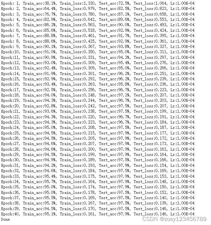
test acc在23 epoch时达到100%
在这里插入图片描述

六、总结与心得

本次手动搭建的vgg16已经达到较高的训练准确率，为99.6%
巩固调用官方模型的操作
在手动搭建的模型基础上进行轻量化，修改后参数数量为121,736,996，并可达到最高训练准确率为100%
感觉自己经过每周的学习，对代码和模型优化更加熟练

zoey123456789

关注

7
点赞
踩
13

收藏

觉得还不错? 一键收藏
0
评论
P7周:基于pytorch的咖啡豆识别-(VGG16复现)

本次手动搭建的vgg16已经达到较高的训练准确率，为99.6%巩固调用官方模型的操作在手动搭建的模型基础上进行轻量化，修改后参数数量为121,736,996，并可达到最高训练准确率为100%感觉自己经过每周的学习，对代码和模型优化更加熟练。
复制链接

扫一扫