How a Kalman filter works, in pictures | Bzarg

原文出自Bzarg的英文博客，看完之后觉得条理清楚，有理有据，故分享。

原文地址： http://www.bzarg.com/p/how-a-kalman-filter-works-in-pictures/

---

I have to tell you about the Kalman filter, because what it does is pretty damn amazing.

Surprisingly few software engineers and scientists seem to know about it, and that makes me sad because it is such a general and powerful tool for combining information in the presence of uncertainty. At times its ability to extract accurate information seems almost magical— and if it sounds like I’m talking this up too much, then take a look at this previously posted video where I demonstrate a Kalman filter figuring out the orientation of a free-floating body by looking at its velocity. Totally neat!

What is it?

You can use a Kalman filter in any place where you have uncertain information about some dynamic system, and you can make an educated guess about what the system is going to do next. Even if messy reality comes along and interferes with the clean motion you guessed about, the Kalman filter will often do a very good job of figuring out what actually happened. And it can take advantage of correlations between crazy phenomena that you maybe wouldn’t have thought to exploit!

Kalman filters are ideal for systems which are continuously changing. They have the advantage that they are light on memory (they don’t need to keep any history other than the previous state), and they are very fast, making them well suited for real time problems and embedded systems.

The math for implementing the Kalman filter appears pretty scary and opaque in most places you find on Google. That’s a bad state of affairs, because the Kalman filter is actually super simple and easy to understand if you look at it in the right way. Thus it makes a great article topic, and I will attempt to illuminate it with lots of clear, pretty pictures and colors. The prerequisites are simple; all you need is a basic understanding of probability and matrices.

I’ll start with a loose example of the kind of thing a Kalman filter can solve, but if you want to get right to the shiny pictures and math, feel free to jump ahead.

What can we do with a Kalman filter?

Let’s make a toy example: You’ve built a little robot that can wander around in the woods, and the robot needs to know exactly where it is so that it can navigate.

We’ll say our robot has a state xk→ , which is just a position and a velocity:

xk→=(p⃗ ,v⃗ )

Note that the state is just a list of numbers about the underlying configuration of your system; it could be anything. In our example it’s position and velocity, but it could be data about the amount of fluid in a tank, the temperature of a car engine, the position of a user’s finger on a touchpad, or any number of things you need to keep track of.

Our robot also has a GPS sensor, which is accurate to about 10 meters, which is good, but it needs to know its location more precisely than 10 meters. There are lots of gullies and cliffs in these woods, and if the robot is wrong by more than a few feet, it could fall off a cliff. So GPS by itself is not good enough.

We might also know something about how the robot moves: It knows the commands sent to the wheel motors, and its knows that if it’s headed in one direction and nothing interferes, at the next instant it will likely be further along that same direction. But of course it doesn’t know everything about its motion: It might be buffeted by the wind, the wheels might slip a little bit, or roll over bumpy terrain; so the amount the wheels have turned might not exactly represent how far the robot has actually traveled, and the prediction won’t be perfect.

The GPS sensor tells us something about the state, but only indirectly, and with some uncertainty or inaccuracy. Our prediction tells us something about how the robot is moving, but only indirectly, and with some uncertainty or inaccuracy.

But if we use all the information available to us, can we get a better answer than either estimate would give us by itself? Of course the answer is yes, and that’s what a Kalman filter is for.

How a Kalman filter sees your problem

Let’s look at the landscape we’re trying to interpret. We’ll continue with a simple state having only position and velocity.

x⃗ =[pv]

We don’t know what the actual position and velocity are; there are a whole range of possible combinations of position and velocity that might be true, but some of them are more likely than others:

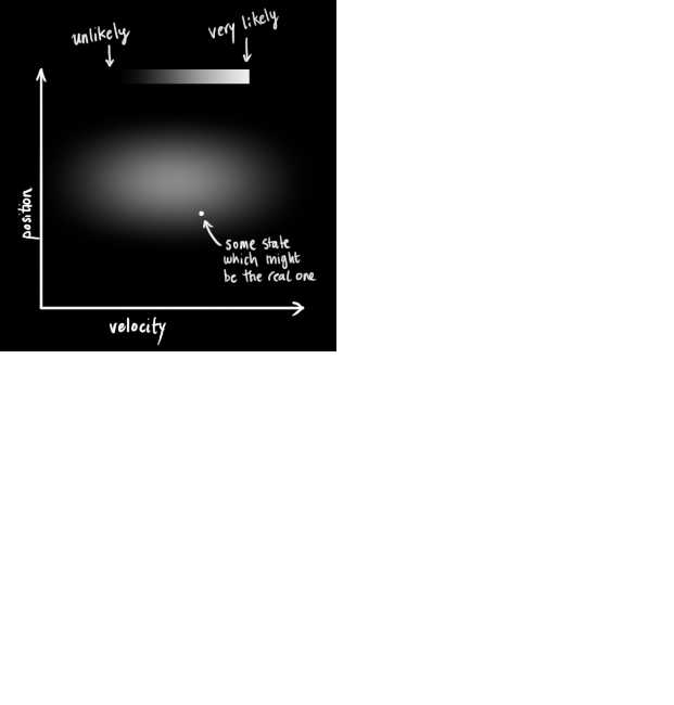
The Kalman filter assumes that both variables (postion and velocity, in our case) are random and Gaussian distributed. Each variable has a mean value μ , which is the center of the random distribution (and its most likely state), and a variance σ2 , which is the uncertainty:

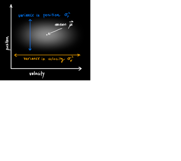
In the above picture, position and velocity are uncorrelated, which means that the state of one variable tells you nothing about what the other might be.

The example below shows something more interesting: Position and velocity are correlated. The likelihood of observing a particular position depends on what velocity you have:

This kind of situation might arise if, for example, we are estimating a new position based on an old one. If our velocity was high, we probably moved farther, so our position will be more distant. If we’re moving slowly, we didn’t get as far.

This kind of relationship is really important to keep track of, because it gives us more information: One measurement tells us something about what the others could be. And that’s the goal of the Kalman filter, we want to squeeze as much information from our uncertain measurements as we possibly can!

This correlation is captured by something called a covariance matrix. In short, each element of the matrix Σij is the degree of correlation between the ith state variable and the jth state variable. (You might be able to guess that the covariance matrix is symmetric, which means that it doesn’t matter if you swap i and j). Covariance matrices are often labelled “ Σ ”, so we call their elements “ Σij ”.

Describing the problem with matrices

We’re modeling our knowledge about the state as a Gaussian blob, so we need two pieces of information at time k : We’ll call our best estimate x^k (the mean, elsewhere named μ ), and its covariance matrix Pk .

x^kPk=[positionvelocity]=[ΣppΣvpΣpvΣvv](1)

(Of course we are using only position and velocity here, but it’s useful to remember that the state can contain any number of variables, and represent anything you want).

Next, we need some way to look at the current state (at time k-1) and predict the next state at time k. Remember, we don’t know which state is the “real” one, but our prediction function doesn’t care. It just works on all of them, and gives us a new distribution:

We can represent this prediction step with a matrix, Fk :

It takes every point in our original estimate and moves it to a new predicted location, which is where the system would move if that original estimate was the right one.

Let’s apply this. How would we use a matrix to predict the position and velocity at the next moment in the future? We’ll use a really basic kinematic formula:

pkvk=pk−1+Δt=vk−1vk−1

In other words:

x^k=[10Δt1]x^k−1=Fkx^k−1(2)(3)

We now have a prediction matrix which gives us our next state, but we still don’t know how to update the covariance matrix.

This is where we need another formula. If we multiply every point in a distribution by a matrix A , then what happens to its covariance matrix Σ ?

Well, it’s easy. I’ll just give you the identity:

Cov(x)Cov(Ax)=Σ=AΣAT(4)

So combining (4)<