


💥💥💞💞欢迎来到本博客❤️❤️💥💥
🏆博主优势:🌞🌞🌞博客内容尽量做到思维缜密,逻辑清晰,为了方便读者。
⛳️座右铭:行百里者,半于九十。
📋📋📋本文目录如下:🎁🎁🎁
目录
⛳️赠与读者
👨💻做科研,涉及到一个深在的思想系统,需要科研者逻辑缜密,踏实认真,但是不能只是努力,很多时候借力比努力更重要,然后还要有仰望星空的创新点和启发点。当哲学课上老师问你什么是科学,什么是电的时候,不要觉得这些问题搞笑。哲学是科学之母,哲学就是追究终极问题,寻找那些不言自明只有小孩子会问的但是你却回答不出来的问题。建议读者按目录次序逐一浏览,免得骤然跌入幽暗的迷宫找不到来时的路,它不足为你揭示全部问题的答案,但若能让人胸中升起一朵朵疑云,也未尝不会酿成晚霞斑斓的别一番景致,万一它居然给你带来了一场精神世界的苦雨,那就借机洗刷一下原来存放在那儿的“躺平”上的尘埃吧。
或许,雨过云收,神驰的天地更清朗.......🔎🔎🔎
💥1 概述
摘要
本文介绍了一个旨在自主驾驶无人水面车辆(USV)前往一组航点的模型预测控制(MPC)算法。该算法的设计被认为对在海洋环境中遇到的环境干扰具有鲁棒性。
由于本工作旨在作为概念验证,因此对USV和干扰的建模已经简化。对于真实世界的实施,应考虑更准确的建模。
介绍
这项工作是在前一项工作的基础上进行的,前一项工作的目标是自主控制USV通过一组航点。实施了一个带有恒定位置参考(即当前航点)跟踪的MPC算法,但这种控制方案并未取得良好的跟踪性能。问题可能源于在全局坐标系中对位置变量进行的优化是非线性的。因此,决定重新设计MPC策略,使优化更简单,使用角度和前向速度变量(在船舶坐标系中完全线性的表达)进入优化问题。
在这个新版本中,算法试图在恒定的时间范围内跟踪角度和前向速度的参考值。船舶模型以更简单但准确的方式重新编写,并编写了一个“智能”参考提供算法,使系统对干扰更具鲁棒性。
首先将讨论USV的建模,然后是使用的跟踪策略。接着将解释参考提供算法(包括处理干扰),最后将介绍MPC算法和所获得的结果。
USV建模
本部分解释了用于描述USV行为的物理学,并说明了如何对其进行建模以便用于MPC方案。
物理描述
所研究的USV具有类似双体船的结构,每个船体末端都有两个固定的推进器。
下图提供了船只及作用于其上的力的图形视图。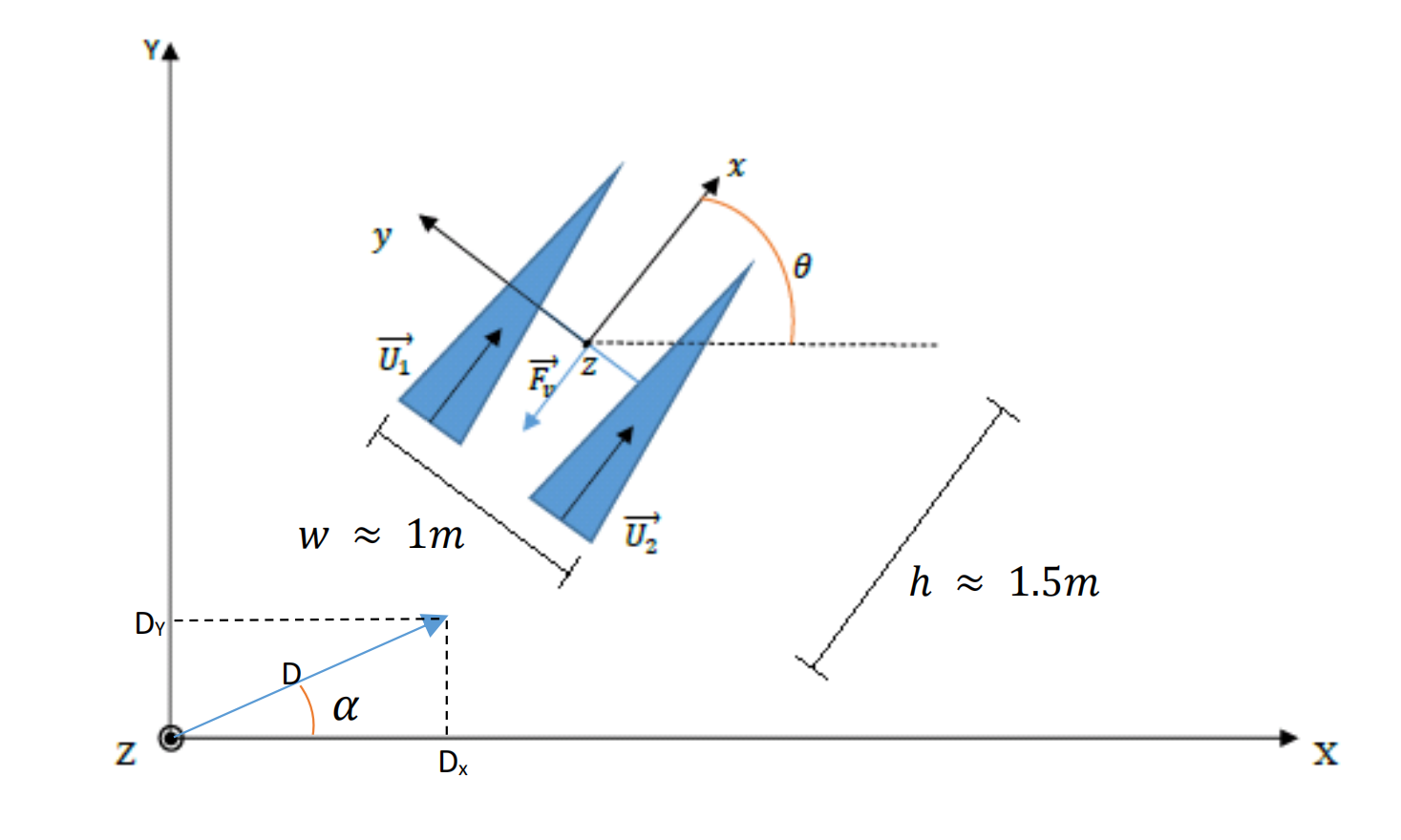
跟踪
之前的部分涉及船只本地坐标系中描述的变量。但为了将船只驶向航点,需要估计船只的位置 - 或进行测量。为了实现这一点,使用了一种称为“死航行”(dead reckoning)的技术。
死航行
技术上讲,死航行等同于在一个时间步长内对船只的速度进行积分,初始条件为实际位置。
由于船只的速度是在其自身的本地坐标系中获得的,因此其在全局坐标系中的位置取决于船只的角度。
同样,将使用状态空间系统来实现这一点。然而,这个系统将是非线性的。
MPC算法
本部分将描述MPC算法以及如何在Matlab中实现它。
之前的MPC控制方案是优化船只在平面上的位置,以驱动它到达下一个航点。这种方法并未取得良好的结果,因为轨迹在任何意义上都不是最佳的。
可能是由于一个糟糕的优化问题引起的,因为船只在全局平面上的位置是由一个非线性系统给出的 - 这是由于船只坐标系和全局坐标系之间的参考框架变换。
因此,决定使用在船只坐标系中轻松表达的变量。注意到船只的角度和巡航速度应该足以控制船只。由于它们可以在船只坐标系中轻松表达,它们应该提供一个更易处理的优化问题。
在建模部分描述的扩展状态空间系统将用于MPC算法 - 加入了干扰的𝐷𝑥项。即使已经用于非扩展系统,标准的𝐴、𝐵符号也将用于其矩阵。
结果
本部分将展示根据本文描述的MPC算法获得的结果。
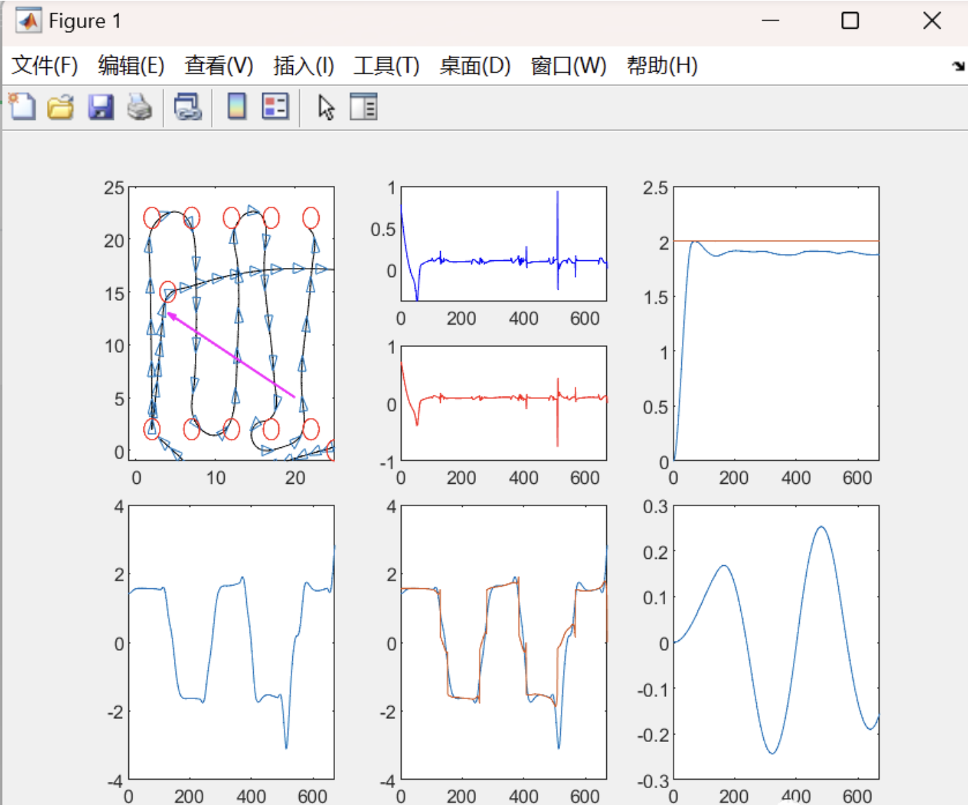
用于验证该算法的仿真基于包含10个航点的基准轨迹。USV必须按照规定顺序到达这10个航点。这个测试已经在有干扰和无干扰的情况下进行过 - 在第二个图中,粉色箭头表示干扰的方向。
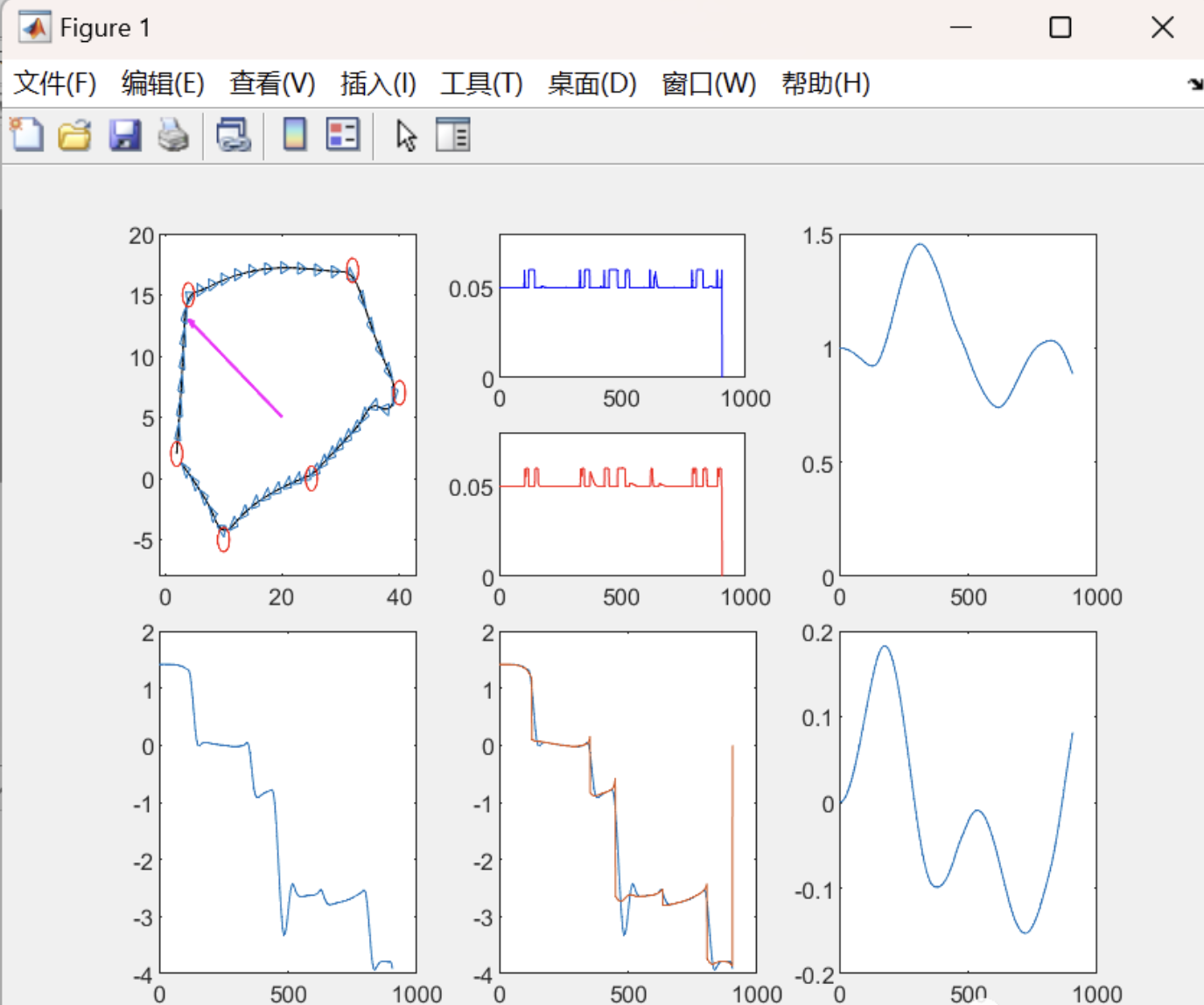
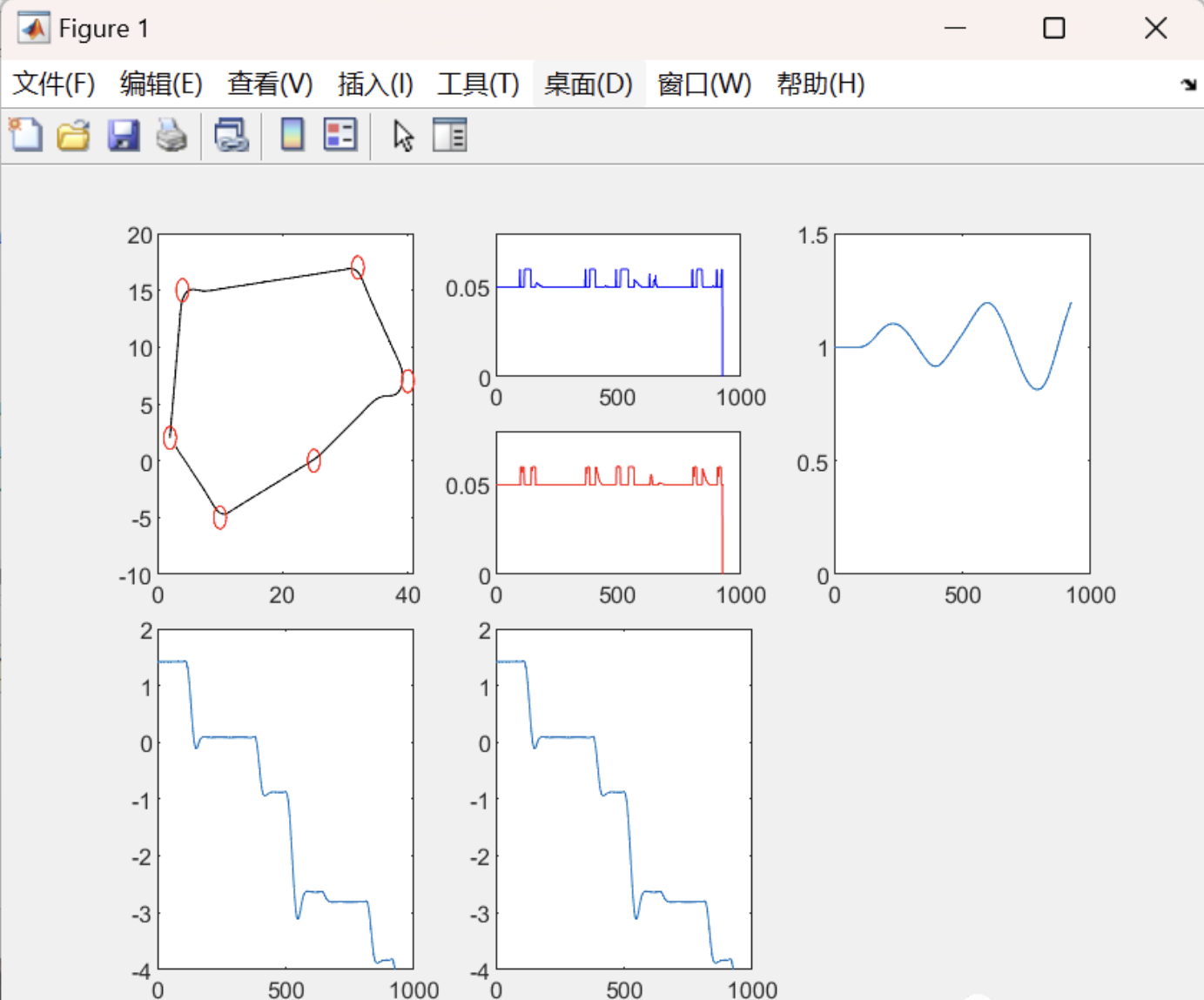
下面的图中从左到右、从上到下分别表示:USV轨迹与航点、施加在每个电机上的推力、前进速度及其参考值、用于提供算法参考的状态向量中的角度、用于MPC算法的状态向量中的角度和𝑦轴船只速度。
在下面的第一个图中 - 无干扰的仿真 - 主要目标显然已经实现:算法以相当优化的方式驱动船只绕过所有航点。然而,观察到船只前进速度存在偏差 - 添加积分增益可能会解决这个问题。并且在第1000个时间步骤左右出现了一个无法解释的角度漂移。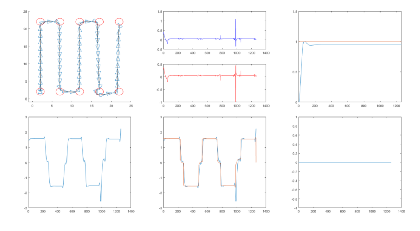
在第二张图中 - 有干扰的仿真 - 主要目标同样已经被清晰地实现。然而,除了前面段落中指出的两个问题外,还出现了另外两个问题:由于与“最佳”路径的距离没有被优化,MPC算法并不关心其轨迹,只要所有航点都被到达,从而导致非最佳轨迹。此外,船只的𝑦轴速度不是一个优化标准,因此所有干扰都通过MPC直接影响船只。问题在于两个电机的角度不可控制,使得校正𝑦轴速度变得困难。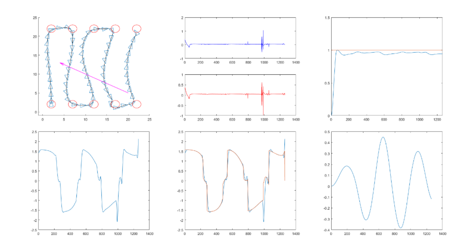
详细文档及数学模型见第4部分。
📚2 运行结果
部分代码:
%%%%%%%%%%% - Clean the workspace and close the open figures - %%%%%%%%%%%%
clear
%close all
%%%%%%%%%%%%%%%%%%% - Boat and simulation parameters - %%%%%%%%%%%%%%%%%%%%
m = 37; %Mass of the boat
D = 0.7; %Distance between the motors and the center of mass
I = 0.1; %Moment of inertia (arbitrary value, should be identified)
k = 0.1; %Viscosity coefficient (arbitrary value, should be identified)
Tfinal = 150; %Total simulation time
Te = 0.1; %Sampling period
V_cruise = 2; %Cruise velocity
i = 1; %Loop index
l = 1; %Boat width
h = 1.5; %Boat height
%%%%%%%%%%%%%%% - Vectors used to hold simulation data - %%%%%%%%%%%%%%%%%%
x = zeros(9, ceil(Tfinal/Te)); %State vector for angle reference
u = zeros(2, ceil(Tfinal/Te)); %Input vector
delta_u = zeros(2, ceil(Tfinal/Te)); %Input increment vector
a = zeros(5, ceil(Tfinal/Te)); %State vector for MPC
a_ref = zeros(1, ceil(Tfinal/Te)); %Angle reference
%%%%%%%%%%%%%%%%%%%%%%%%% - Mission planning - %%%%%%%%%%%%%%%%%%%%%%%%%%%%
%x_list = [2 4 32 40 25 10 2]'; %X coordinates of the waypoints
%y_list = [2 15 17 7 0 -5 2]'; %Y coordinates of the waypoints
x_list = [2 2 7 7 12 12 17 17 22 22]';
y_list = [2 22 22 2 2 22 22 2 2 22]';
nb_obj = size(x_list,1); %Number of objectives
r_list = [x_list y_list]; %Objective list containing X and Y data
current_obj = 2; %As the boat starts in the first
%waypoint, the current objective is 2
%%%%%%%%%%%%%%% - State-space system used for the MPC - %%%%%%%%%%%%%%%%%%%
%Initial conditions
a(:,i) = [0 0 1.4181 0 0]'; %Initial state vector
u(:,i) = [0 0]'; %Initial input vector
delta_u(:,i) = [0 0]'; %Initial input increment vector
%System matrices
A = [1 0 0 0 0;... %State matrix
Te 1 0 0 0;...
0 Te 1 0 0;...
0 0 0 1 Te;...
0 0 0 -k/m 1];
B = [D/(2*I) -D/(2*I);... %Input matrix
0 0; 0 0; 0 0; 1/m 1/m];
n_input = size(B,2); %Number of inputs
n_state = size(B,1); %Number of state variables
%Augmented system matrices
A_tilde = [A B; zeros(n_input,n_state), eye(n_input)]; %State matrix
B_tilde = [zeros(n_state,n_input); eye(n_input)]; %Input matrix
C_tilde = [0 0 1 0 0 0 0;... %Output matrix
0 0 0 1 0 0 0];
n_output = size(C_tilde,1); %Number of outputs
%%%%% - State-space system used to provide an angle reference vector - %%%%
x(:,i) = [2 2 1.4181 0 0 0 0 0 0]'; %Initial state vector
%Linearized state matrix
Fx = [1 0 0 0 0 Te*cos(x(3,i)) 0 -Te*sin(x(3,i)) 0;...
0 1 0 0 0 Te*sin(x(3,i)) 0 Te*cos(x(3,i)) 0;...
0 0 1 Te 0 0 0 0 0;...
0 0 0 1 Te 0 0 0 0;...
0 0 0 0 1 0 0 0 0;...
0 0 0 0 0 1 Te 0 0;...
0 0 0 0 0 -k/m 1 0 0;...
0 0 0 0 0 0 0 1 Te;...
0 0 0 0 0 0 0 -k/m 1];
%Linearized input matrix
Fu = [0 0; 0 0; 0 0; 0 0;...
D/(2*I) -D/(2*I); 0 0; 1/m 1/m; 0 0; 0 0];
%%%%%%%%%%%%%%%%%%%%%% - Disturbances modeling - %%%%%%%%%%%%%%%%%%%%%%%%%%
Dx = -0.02; %Disturbance surge on the X axis
Dy = 0.01; %Disturbance surge on the Y axis
alpha = angle(complex(Dx,Dy)); %Angle of the disturbance vector
Dk = [0 0 0 0 0 0 ... %Disturbance vector
(1/m)*Dx*cos(alpha-x(3,i)) 0 (1/m)*Dy*sin(alpha-x(3,i))]';
%%%%%%%%%%%%%%%%%%%%%%%%%% - MPC parameters - %%%%%%%%%%%%%%%%%%%%%%%%%%%%%
nu = 2; %Control horizon
ny = 30; %Prediction horizon
r = zeros(n_output*ny,1); %Angle reference vector
%Matrices used for optimization
gainS = computeGainS(n_output, 1); %Steady-state gain
gainQ = computeGainQ(n_output, [2 0;0 1]); %Outputs running cost gain
gainR = computeGainR(n_input, 1); %Inputs running cost gain
Qbar = computeQbar(C_tilde, gainQ, gainS, ny);
Tbar = computeTbar(gainQ, C_tilde, gainS, ny);
Rbar = computeRbar(gainR, nu);
Cbar = computeCbar(A_tilde, B_tilde, ny, nu);
Abar = computeAbar(A_tilde, ny);
Hbar = computeHbar(Cbar, Qbar, Rbar);
Fbar = computeFbar(Abar, Qbar, Cbar, Tbar);
%State constraints vectors
%[theta_dot_dot theta_dot theta x_dot x_dot_dot U1 U2]
Cmin = [-100 -100 -2*pi 0 -10000 -1000*k/2 -1000*k/2]';
Cmax = [100 100 2*pi V_cruise 10000 1000*k/2 1000*k/2]';
%Quadprog solver options
%Keep the solver quiet
options = optimoptions('quadprog');
options = optimoptions(options, 'Display', 'off');
%Simulation loop
for t=0:Te:(Tfinal-1)
a_tilde = [a(:,i); u(:,i)]; %Augmented state vector for MPC
%Compute the ny next angle objectives
tmp = x(:,i); %Get the current state
obj = current_obj; %Get the current objective
j = 1;
while(j <= n_output*ny)
%Compute the angle of the line between the boat and the waypoint
goal_angle = angle(complex(r_list(obj,1)-tmp(1,1), r_list(obj,2)-tmp(2,1)));
%If the distance between the goal angle and the current angle is
%greater than pi, it means that there is a shorter path to this
%angle than getting all the way around the unit circle
dist = abs(goal_angle - tmp(3,1));
if dist > pi
if tmp(3,1) < 0
goal_angle = tmp(3,1) - (2*pi - dist);
else
goal_angle = tmp(3,1) + (2*pi - dist);
end
end
%Considering an optimal orientation of the boat and equal inputs
%compute the Ny next boat position.
%If the boat is not yet arrived to the waypoint put the goal_angle
%into the reference vector, else recompute the goal angle.
tmp(3,1) = goal_angle;
%Make sure we're using the right state and disturbance matrices
Fx = [1 0 0 0 0 Te*cos(tmp(3,1)) 0 -Te*sin(tmp(3,1)) 0;...
0 1 0 0 0 Te*sin(tmp(3,1)) 0 Te*cos(tmp(3,1)) 0;...
0 0 1 Te 0 0 0 0 0;...
0 0 0 1 Te 0 0 0 0;...
0 0 0 0 1 0 0 0 0;...
0 0 0 0 0 1 Te 0 0;...
0 0 0 0 0 -k/m 1 0 0;...
0 0 0 0 0 0 0 1 Te;...
0 0 0 0 0 0 0 -k/m 1];
Dk = [0 0 0 0 0 0 (1/m)*Dx*cos(alpha-tmp(3,1)) ...
0 (1/m)*Dy*sin(alpha-tmp(3,1))]';
%Make a step forward
tmp = Fx*tmp + Fu*(V_cruise*[k/2;k/2]) + Dk;
%Have we reached the next waypoint ?
if(tmp(1) > r_list(obj,1) - 0.5 && tmp(1) < r_list(obj,1) + 0.5 && ...
tmp(2) > r_list(obj,2) - 0.5 && tmp(2) < r_list(obj,2) + 0.5)
%If yes, update the objective
obj = mod(obj,7) + 1;
🎉3 参考文献
文章中一些内容引自网络,会注明出处或引用为参考文献,难免有未尽之处,如有不妥,请随时联系删除。
[1]杨瑞雯,刘宇晨,张宇飞,等.基于模型预测的无人车辆自主控制仿真研究[J].计算机仿真, 2023(008):040.
[2]柳晨光. 基于预测控制的无人船运动控制方法研究[D]. 武汉理工大学.


 1419
1419


 被折叠的 条评论
为什么被折叠?
被折叠的 条评论
为什么被折叠?
 到【灌水乐园】发言


