个人学习笔记7-3：动手学深度学习pytorch版-李沐

#深度学习# #人工智能# #神经网络# #计算机视觉# #python#

计算机视觉

13.7 单发多框检测（SSD）

SSD模型主要由基础网络组成，其后是几个多尺度特征块。

SSD通过单神经网络来检测模型，以每个像素为中心的产生多个锚框，在多个段的输出上进行多尺度的检测。

##

补充YOLO:

##

SSD实现：

类别预测层:

我们定义了这样一个类别预测层，通过参数num_anchors和num_classes分别指定了𝑎和𝑞。 该图层使用填充为1的3×33×3的卷积层。此卷积层的输入和输出的宽度和高度保持不变。

%matplotlib inline
import torch
import torchvision
from torch import nn
from torch.nn import functional as F
from d2l import torch as d2l


def cls_predictor(num_inputs, num_anchors, num_classes):
    return nn.Conv2d(num_inputs, num_anchors * (num_classes + 1),
                     kernel_size=3, padding=1)

边界框预测层:

边界框预测层的设计与类别预测层的设计类似。 唯一不同的是，这里需要为每个锚框预测4个偏移量，而不是𝑞+1个类别。

def bbox_predictor(num_inputs, num_anchors):
    return nn.Conv2d(num_inputs, num_anchors * 4, kernel_size=3, padding=1)

连结多尺度的预测:

单发多框检测使用多尺度特征图来生成锚框并预测其类别和偏移量。 在不同的尺度下，特征图的形状或以同一单元为中心的锚框的数量可能会有所不同。 因此，不同尺度下预测输出的形状可能会有所不同。验证如下：

def forward(x, block):
    return block(x)

Y1 = forward(torch.zeros((2, 8, 20, 20)), cls_predictor(8, 5, 10))
Y2 = forward(torch.zeros((2, 16, 10, 10)), cls_predictor(16, 3, 10))
Y1.shape, Y2.shape

结果输出：

除了批量大小这一维度外，其他三个维度都具有不同的尺寸。为了将这两个预测输出链接起来以提高计算效率，我们将把这些张量转换为更一致的格式。通道维包含中心相同的锚框的预测结果。我们首先将通道维移到最后一维。 因为不同尺度下批量大小仍保持不变，我们可以将预测结果转成二维的（批量大小，高××宽××通道数）的格式，以方便之后在维度11上的连结。

def flatten_pred(pred):
    return torch.flatten(pred.permute(0, 2, 3, 1), start_dim=1)

def concat_preds(preds):
    return torch.cat([flatten_pred(p) for p in preds], dim=1)

现，尽管Y1和Y2在通道数、高度和宽度方面具有不同的大小，我们仍然可以在同一个小批量的两个不同尺度上连接这两个预测输出。

concat_preds([Y1, Y2]).shape

结果输出：

高和宽减半块：

定义了高和宽减半块down_sample_blk，该模块将输入特征图的高度和宽度减半。

def down_sample_blk(in_channels, out_channels):
    blk = []
    for _ in range(2):
        blk.append(nn.Conv2d(in_channels, out_channels,
                             kernel_size=3, padding=1))
        blk.append(nn.BatchNorm2d(out_channels))
        blk.append(nn.ReLU())
        in_channels = out_channels
    blk.append(nn.MaxPool2d(2))
    return nn.Sequential(*blk)

示例，我们构建的高和宽减半块会更改输入通道的数量，并将输入特征图的高度和宽度减半。

forward(torch.zeros((2, 3, 20, 20)), down_sample_blk(3, 10)).shape

结果输出：

基本网络块：

基本网络块用于从输入图像中抽取特征：

def base_net():
    blk = []
    num_filters = [3, 16, 32, 64]
    for i in range(len(num_filters) - 1):
        blk.append(down_sample_blk(num_filters[i], num_filters[i+1]))
    return nn.Sequential(*blk)

forward(torch.zeros((2, 3, 256, 256)), base_net()).shape

结果输出：

完整的模型：

def get_blk(i):
    if i == 0:
        blk = base_net()
    elif i == 1:
        blk = down_sample_blk(64, 128)
    elif i == 4:
        blk = nn.AdaptiveMaxPool2d((1,1))
    else:
        blk = down_sample_blk(128, 128)
    return blk

为每个块定义前向传播。与图像分类任务不同，此处的输出包括：CNN特征图Y；在当前尺度下根
据Y生成的锚框；预测的这些锚框的类别和偏移量（基于Y）。

def blk_forward(X, blk, size, ratio, cls_predictor, bbox_predictor):
    Y = blk(X)
    anchors = d2l.multibox_prior(Y, sizes=size, ratios=ratio)
    cls_preds = cls_predictor(Y)
    bbox_preds = bbox_predictor(Y)
    return (Y, anchors, cls_preds, bbox_preds)

超参数：

sizes = [[0.2, 0.272], [0.37, 0.447], [0.54, 0.619], [0.71, 0.79],
         [0.88, 0.961]]
ratios = [[1, 2, 0.5]] * 5
num_anchors = len(sizes[0]) + len(ratios[0]) - 1

定义完整的模型TinySSD：

class TinySSD(nn.Module):
    def __init__(self, num_classes, **kwargs):
        super(TinySSD, self).__init__(**kwargs)
        self.num_classes = num_classes
        idx_to_in_channels = [64, 128, 128, 128, 128]
        for i in range(5):
            # 即赋值语句self.blk_i=get_blk(i)
            setattr(self, f'blk_{i}', get_blk(i))
            setattr(self, f'cls_{i}', cls_predictor(idx_to_in_channels[i],
                                                    num_anchors, num_classes))
            setattr(self, f'bbox_{i}', bbox_predictor(idx_to_in_channels[i],
                                                      num_anchors))

    def forward(self, X):
        anchors, cls_preds, bbox_preds = [None] * 5, [None] * 5, [None] * 5
        for i in range(5):
            # getattr(self,'blk_%d'%i)即访问self.blk_i
            X, anchors[i], cls_preds[i], bbox_preds[i] = blk_forward(
                X, getattr(self, f'blk_{i}'), sizes[i], ratios[i],
                getattr(self, f'cls_{i}'), getattr(self, f'bbox_{i}'))
        anchors = torch.cat(anchors, dim=1)
        cls_preds = concat_preds(cls_preds)
        cls_preds = cls_preds.reshape(
            cls_preds.shape[0], -1, self.num_classes + 1)
        bbox_preds = concat_preds(bbox_preds)
        return anchors, cls_preds, bbox_preds

创建一个模型实例，然后使用它对一个256 × 256像素的小批量图像X执行前向传播：

net = TinySSD(num_classes=1)
X = torch.zeros((32, 3, 256, 256))
anchors, cls_preds, bbox_preds = net(X)

print('output anchors:', anchors.shape)
print('output class preds:', cls_preds.shape)
print('output bbox preds:', bbox_preds.shape)

结果输出：

13.7.2 训练模型

读取数据集和初始化：

batch_size = 32
train_iter, _ = d2l.load_data_bananas(batch_size)

初始化其参数并定义优化算法：

device, net = d2l.try_gpu(), TinySSD(num_classes=1)
trainer = torch.optim.SGD(net.parameters(), lr=0.2, weight_decay=5e-4)

定义损失函数和评价函数：

cls_loss = nn.CrossEntropyLoss(reduction='none')
bbox_loss = nn.L1Loss(reduction='none')

def calc_loss(cls_preds, cls_labels, bbox_preds, bbox_labels, bbox_masks):
    batch_size, num_classes = cls_preds.shape[0], cls_preds.shape[2]
    cls = cls_loss(cls_preds.reshape(-1, num_classes),
                   cls_labels.reshape(-1)).reshape(batch_size, -1).mean(dim=1)
    bbox = bbox_loss(bbox_preds * bbox_masks,
                     bbox_labels * bbox_masks).mean(dim=1)
    return cls + bbox

使用平均绝对误差来评价边界框的预测结果：

def cls_eval(cls_preds, cls_labels):
    # 由于类别预测结果放在最后一维，argmax需要指定最后一维。
    return float((cls_preds.argmax(dim=-1).type(
        cls_labels.dtype) == cls_labels).sum())

def bbox_eval(bbox_preds, bbox_labels, bbox_masks):
    return float((torch.abs((bbox_labels - bbox_preds) * bbox_masks)).sum())

训练模型：

num_epochs, timer = 50, d2l.Timer()
animator = d2l.Animator(xlabel='epoch', xlim=[1, num_epochs],
                        legend=['class error', 'bbox mae'])
net = net.to(device)
for epoch in range(num_epochs):
    # 训练精确度的和，训练精确度的和中的示例数
    # 绝对误差的和，绝对误差的和中的示例数
    metric = d2l.Accumulator(4)
    net.train()
    for features, target in train_iter:
        timer.start()
        trainer.zero_grad()
        X, Y = features.to(device), target.to(device)
        # 生成多尺度的锚框，为每个锚框预测类别和偏移量
        anchors, cls_preds, bbox_preds = net(X)
        # 为每个锚框标注类别和偏移量
        bbox_labels, bbox_masks, cls_labels = d2l.multibox_target(anchors, Y)
        # 根据类别和偏移量的预测和标注值计算损失函数
        l = calc_loss(cls_preds, cls_labels, bbox_preds, bbox_labels,
                      bbox_masks)
        l.mean().backward()
        trainer.step()
        metric.add(cls_eval(cls_preds, cls_labels), cls_labels.numel(),
                   bbox_eval(bbox_preds, bbox_labels, bbox_masks),
                   bbox_labels.numel())
    cls_err, bbox_mae = 1 - metric[0] / metric[1], metric[2] / metric[3]
    animator.add(epoch + 1, (cls_err, bbox_mae))
print(f'class err {cls_err:.2e}, bbox mae {bbox_mae:.2e}')
print(f'{len(train_iter.dataset) / timer.stop():.1f} examples/sec on '
      f'{str(device)}')

结果输出：

13.7.3 预测目标

我们读取并调整测试图像的大小，然后将其转成卷积层需要的四维格式：

X = torchvision.io.read_image('../img/banana.jpg').unsqueeze(0).float()
img = X.squeeze(0).permute(1, 2, 0).long()

使用下面的multibox_detection函数，我们可以根据锚框及其预测偏移量得到预测边界框。然后，通过非极大值抑制来移除相似的预测边界框。

def predict(X):
    net.eval()
    anchors, cls_preds, bbox_preds = net(X.to(device))
    cls_probs = F.softmax(cls_preds, dim=2).permute(0, 2, 1)
    output = d2l.multibox_detection(cls_probs, bbox_preds, anchors)
    idx = [i for i, row in enumerate(output[0]) if row[0] != -1]
    return output[0, idx]

output = predict(X)

所有置信度不低于0.9的边界框，做为最终输出：

def display(img, output, threshold):
    d2l.set_figsize((5, 5))
    fig = d2l.plt.imshow(img)
    for row in output:
        score = float(row[1])
        if score < threshold:
            continue
        h, w = img.shape[0:2]
        bbox = [row[2:6] * torch.tensor((w, h, w, h), device=row.device)]
        d2l.show_bboxes(fig.axes, bbox, '%.2f' % score, 'w')

display(img, output.cpu(), threshold=0.9)

结果输出：（等GPU出结果）

13.8 区域卷积神经网络（R-CNN）系列

区域卷积神经网络（region‐based CNN或regions with CNN features，R‐CNN）是将深度模型应用于目标检测的开创性工作之一。本节将介绍R‐CNN及其一系列改进方法：快速的R‐CNN（Fast R‐CNN）、更快的R‐CNN（Faster R‐CNN）和掩码R‐CNN（Mask R‐CNN）。

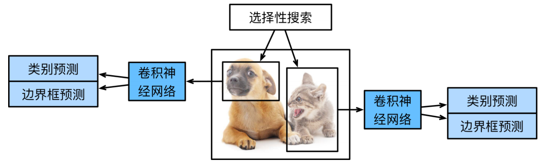
13.8.1 R-CNN

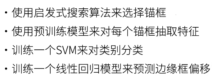
R-CNN首先从输入图像中选取若干个提议区域（如锚框也是一种选取方法），并标注它们的类别和边界框（如偏移量）。然后，用卷积神经网络对每个提议区域进行前向传播以抽取其特征。接下来，我们用每个提议区域的特征来预测类别和边界框。（后续计划详细研究论文再补充）

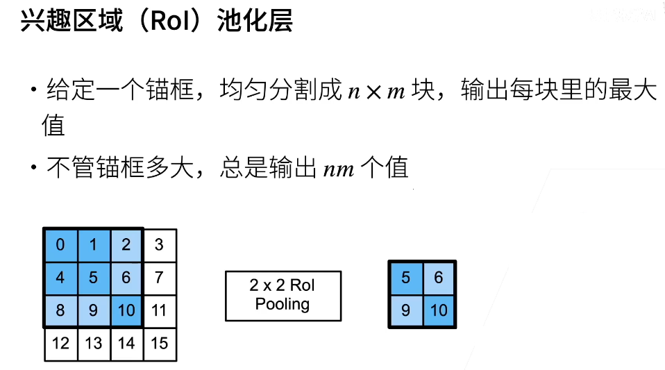
问题：锚框每次选到的大小不一样，怎么样使得这些锚框最后可以变成一个batch。用rol池化层解决。

兴趣区域池化层（region of interest pooling，RoI 池化层）：（下图中黑色为锚框，要输出2x2；则不均匀划分，输出每个部分最大值）

13.8.2 Fast R-CNN

R‐CNN的主要性能瓶颈在于，对每个提议区域，卷积神经网络的前向传播是独立的，而没有共享计算。由于这些区域通常有重叠，独立的特征抽取会导致重复的计算。Fast R-CNN 是对R‐CNN的主要改进之一，是仅在整张图象上执行卷积神经网络的前向传播。（后续计划详细研究论文再补充）

13.8.3 Faster R-CNN

为了较精确地检测目标结果，Fast R‐CNN模型通常需要在选择性搜索中生成大量的提议区域。Faster R-CNN提出将选择性搜索替换为区域提议网络（region proposal network），从而减少提议区域的生成数量，并保证目标检测的精度。（后续计划详细研究论文再补充）

13.8.4 Mask R-CNN

Mask R‐CNN是基于Faster R‐CNN修改而来的，Mask R‐CNN将兴趣区域汇聚层替换为了 兴趣区域对齐层，使用双线性插值（bilinear interpolation）来保留特征图上的空间信息，从而更适于像素级预测。