机器学习：Softmax回归（Python）

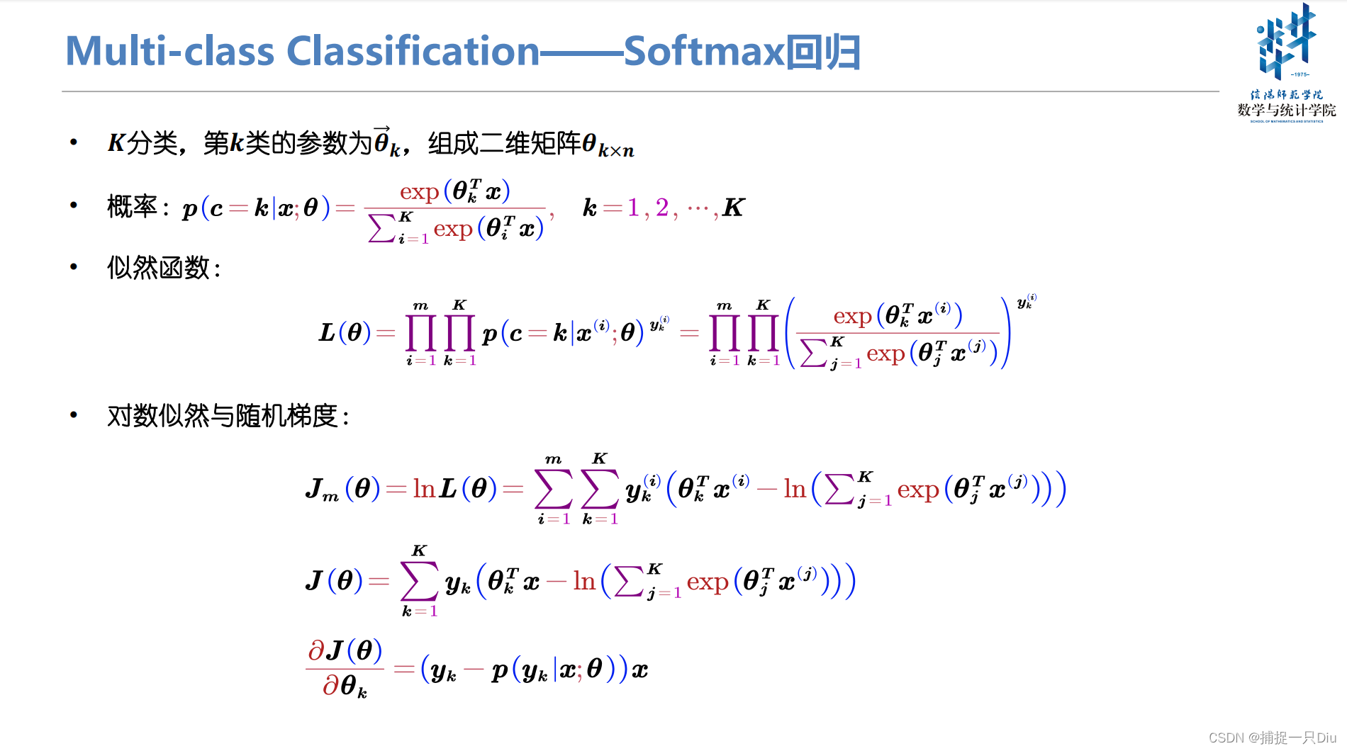
Softmax回归（多分类）

logistic_regression_mulclass.py

import numpy as np
import matplotlib.pyplot as plt


class LogisticRegression_MulClass:
    """
    逻辑回归，采用梯度下降算法 + 正则化，交叉熵损失函数，实现多分类，Softmax函数
    """
    def __init__(self, fit_intercept=True, normalize=True, alpha=0.05, eps=1e-10,
                 max_epochs=300, batch_size=20, l1_ratio=None, l2_ratio=None, en_rou=None):
        """
        :param eps: 提前停止训练的精度要求，按照两次训练损失的绝对值差小于eps，停止训练
        :param fit_intercept: 是否训练偏置项
        :param normalize: 是否标准化
        :param alpha: 学习率
        :param max_epochs: 最大迭代次数
        :param batch_size: 批量大小，若为1，则为随机梯度，若为训练集样本量，则为批量梯度，否则为小批量梯度
        :param l1_ratio: LASSO回归惩罚项系数
        :param l2_ratio: 岭回归惩罚项系数
        :param en_rou: 弹性网络权衡L1和L2的系数
        """
        self.fit_intercept = fit_intercept  # 线性模型的常数项。也即偏置bias，模型中的theta0
        self.normalize = normalize  # 是否标准化数据
        self.alpha = alpha  # 学习率
        self.eps = eps  # 提前停止训练
        if l1_ratio:
            if l1_ratio < 0:
                raise ValueError("惩罚项系数不能为负数")
        self.l1_ratio = l1_ratio  # LASSO回归惩罚项系数
        if l2_ratio:
            if l2_ratio < 0:
                raise ValueError("惩罚项系数不能为负数")
        self.l2_ratio = l2_ratio  # 岭回归惩罚项系数
        if en_rou:
            if en_rou > 1 or en_rou < 0:
                raise ValueError("弹性网络权衡系数范围在[0, 1]")
        self.en_rou = en_rou  # 弹性网络权衡L1和L2的系数
        self.max_epochs = max_epochs
        self.batch_size = batch_size
        self.theta = None  # 训练权重系数
        if normalize:
            self.feature_mean, self.feature_std = None, None  # 特征的均值，标准方差
        self.n_samples, self.n_classes = 0, 0  # 样本量和类别数
        self.train_loss, self.test_loss = [], []  # 存储训练过程中的训练损失和测试损失

    def init_theta_params(self, n_features, n_classes):
        """
        初始化参数
        如果训练偏置项，也包含了bias的初始化
        :param n_features: 样本的特征数量
        :param n_classes: 类别数
        :return: n_features * n_classes
        """
        self.theta = np.random.randn(n_features, n_classes) * 0.05

    @staticmethod
    def one_hot_encoding(target):
        """
        类别编码
        :param target:
        :return:
        """
        class_labels = np.unique(target)  # 类别标签，去重
        target_y = np.zeros((len(target), len(class_labels)), dtype=np.int64)
        for i, label in enumerate(target):
            target_y[i, label] = 1  # 对应类别所在列为1
        return target_y

    @staticmethod
    def softmax_func(x):
        """
        softmax函数，为避免上溢或下溢，对参数x做限制
        :param x: 数组: batch_size * n_classes
        :return:  1 * n_classes
        """
        exps = np.exp(x - np.max(x))  # 避免溢出，每个数减去其最大值
        exp_sum = np.sum(exps, axis=1, keepdims=True)
        return exps / exp_sum


    @staticmethod
    def sign_func(z_values):
        """
        符号函数，针对L1正则化
        :param z_values: 模型系数，二维数组
        :return:
        """
        sign = np.zeros(z_values.shape)
        sign[z_values > 0] = 1.0
        sign[z_values < 0] = -1.0
        return sign

    @staticmethod
    def cal_cross_entropy(y_test, y_prob):
        """
        计算交叉熵损失
        :param y_test: 样本真值，二维数组n * c，c表示类别数
        :param y_prob: 模型预测类别概率，n * c
        :return:
        """
        loss = -np.sum(y_test * np.log(y_prob + 1e-08), axis=1)
        loss -= np.sum((1 - y_test) * np.log(1 - y_prob + 1e-08), axis=1)
        return np.mean(loss)

    def fit(self, x_train, y_train, x_test=None, y_test=None):
        """
        样本的预处理，模型系数的求解，闭式解公式 + 梯度方法
        :param x_train: 训练样本集 m*k
        :param y_train: 训练目标集 m*c
        :param x_test: 测试样本集 n*k
        :param y_test: 测试目标集 n*c
        :return:
        """
        y_train = self.one_hot_encoding(y_train)
        self.n_classes = y_train.shape[1]  # 类别数
        if y_test is not None:
            y_test = self.one_hot_encoding(y_test)
        if self.normalize:
            self.feature_mean = np.mean(x_train, axis=0)  # 样本均值
            self.feature_std = np.std(x_train, axis=0) + 1e-8  # 样本方差
            x_train = (x_train - self.feature_mean) / self.feature_std  # 标准化
            if x_test is not None:
                x_test = (x_test - self.feature_mean) / self.feature_std  # 标准化
        if self.fit_intercept:
            x_train = np.c_[x_train, np.ones((len(y_train), 1))]  # 添加一列1，即偏置项样本
            if x_test is not None and y_test is not None:
                x_test = np.c_[x_test, np.ones((len(y_test), 1))]  # 添加一列1，即偏置项样本
        self.init_theta_params(x_train.shape[1], self.n_classes)  # 初始化参数
        # 训练模型
        self._fit_gradient_desc(x_train, y_train, x_test, y_test)  # 梯度下降法训练模型

    def _fit_gradient_desc(self, x_train, y_train, x_test=None, y_test=None):
        """
        三种梯度下降求解 + 正则化：
        （1）如果batch_size为1，则为随机梯度下降法
        （2）如果batch_size为样本量，则为批量梯度下降法
        （3）如果batch_size小于样本量，则为小批量梯度下降法
        :return:
        """
        train_sample = np.c_[x_train, y_train]  # 组合训练集和目标集，以便随机打乱样本
        # np.c_水平方向连接数组，np.r_竖直方向连接数组
        # 按batch_size更新theta，三种梯度下降法取决于batch_size的大小
        for epoch in range(self.max_epochs):
            self.alpha *= 0.95
            np.random.shuffle(train_sample)  # 打乱样本顺序，模拟随机化
            batch_nums = train_sample.shape[0] // self.batch_size  # 批次
            for idx in range(batch_nums):
                # 取小批量样本，可以是随机梯度（1），批量梯度（n）或者是小批量梯度（<n）
                batch_xy = train_sample[self.batch_size * idx: self.batch_size * (idx + 1)]
                # 分取训练样本和目标样本，注意目标值不再是一列
                batch_x, batch_y = batch_xy[:, :x_train.shape[1]], batch_xy[:, x_train.shape[1]:]
                # 计算权重更新增量，包含偏置项
                y_prob_batch = self.softmax_func(batch_x.dot(self.theta))  # 小批量的预测概率
                # 1 * n <--> n * k = 1 * k --> 转置 k * 1
                delta = ((y_prob_batch - batch_y).T.dot(batch_x) / self.batch_size).T
                # 计算并添加正则化部分，不包含偏置项，最后一列是偏置项
                dw_reg = np.zeros(shape=(x_train.shape[1] - 1, self.n_classes))
                if self.l1_ratio and self.l2_ratio is None:
                    # LASSO回归，L1正则化
                    dw_reg = self.l1_ratio * self.sign_func(self.theta[:-1, :])
                if self.l2_ratio and self.l1_ratio is None:
                    # Ridge回归，L2正则化
                    dw_reg = 2 * self.l2_ratio * self.theta[:-1, :]
                if self.en_rou and self.l1_ratio and self.l2_ratio:
                    # 弹性网络
                    dw_reg = self.l1_ratio * self.en_rou * self.sign_func(self.theta[:-1, :])
                    dw_reg += 2 * self.l2_ratio * (1 - self.en_rou) * self.theta[:-1, :]
                delta[:-1, :] += dw_reg / self.batch_size  # 添加了正则化
                self.theta = self.theta - self.alpha * delta
            # 计算训练过程中的交叉熵损失值
            y_train_prob = self.softmax_func(x_train.dot(self.theta))  # 当前迭代训练的模型预测概率
            train_cost = self.cal_cross_entropy(y_train, y_train_prob)  # 训练集的交叉熵损失
            self.train_loss.append(train_cost)  # 交叉熵损失均值
            if x_test is not None and y_test is not None:
                y_test_prob = self.softmax_func(x_test.dot(self.theta))  # 当前测试样本预测概率
                test_cost = self.cal_cross_entropy(y_test, y_test_prob)
                self.test_loss.append(test_cost)  # 交叉熵损失均值
            # 两次交叉熵损失均值的差异小于给定的均值，提前停止训练
            if epoch > 10 and (np.abs(self.train_loss[-1] - self.train_loss[-2])) <= self.eps:
                break

    def get_params(self):
        """
        返回线性模型训练的系数
        :return:
        """
        if self.fit_intercept:  # 存在偏置项
            weight, bias = self.theta[:-1, :], self.theta[-1, :]
        else:
            weight, bias = self.theta, np.array([0])
        if self.normalize:  # 标准化后的系数
            weight = weight / self.feature_std.reshape(-1, 1)  # 还原模型系数
            bias = bias - weight.T.dot(self.feature_mean)
        return weight, bias

    def predict_prob(self, x_test):
        """
        预测测试样本的概率，第1列为y = 0的概率，第2列是y = 1的概率
        :param x_test: 测试样本，ndarray：n * k
        :return:
        """
        if self.normalize:
            x_test = (x_test - self.feature_mean) / self.feature_std  # 测试数据标准化
        if self.fit_intercept:
            # 存在偏置项，加一列1
            x_test = np.c_[x_test, np.ones(shape=x_test.shape[0])]
        y_prob = self.softmax_func(x_test.dot(self.theta))
        return y_prob

    def predict(self, x):
        """
        预测样本类别
        :param x: 预测样本
        :return:
        """
        y_prob = self.predict_prob(x)
        # 对应每个样本中所有类别的概率，哪个概率大，返回哪个类别所在索引列编号，即类别
        return np.argmax(y_prob, axis=1)

    def plt_loss_curve(self, lab=None, is_show=True):
        """
        可视化交叉熵损失曲线
        :param is_show: 是否可视化
        :return:
        """
        if is_show:
            plt.figure(figsize=(8, 6))
        plt.plot(self.train_loss, "k-", lw=1, label="Train Loss")
        if self.test_loss:
            plt.plot(self.test_loss, "r--", lw=1.2, label="Test Loss")
        plt.xlabel("Training Epochs", fontdict={"fontsize": 12})
        plt.ylabel("The Mean of Cross Entropy Loss", fontdict={"fontsize": 12})
        plt.title("%s: The Loss Curve of Cross Entropy" % lab)
        plt.legend(frameon=False)
        plt.grid(ls=":")
        # plt.axis([0, 300, 20, 30])
        if is_show:
            plt.show()

test_logistic_reg_mulclass.py

from sklearn.datasets import load_breast_cancer, load_iris, load_digits
from sklearn.model_selection import train_test_split
from logistic_regression_mulclass import LogisticRegression_MulClass
import matplotlib.pyplot as plt
from performance_metrics import ModelPerformanceMetrics
from sklearn.preprocessing import StandardScaler


iris = load_iris()  # 加载数据集
X, y = iris.data, iris.target
X = StandardScaler().fit_transform(X)  # 标准化

X_train, X_test, y_train, y_test = train_test_split(X, y, test_size=0.3, random_state=0, stratify=y)

lg_lr = LogisticRegression_MulClass(alpha=0.5, l1_ratio=0.5,
                                    batch_size=5, normalize=False, max_epochs=1000, eps=1e-15)
lg_lr.fit(X_train, y_train, X_test, y_test)

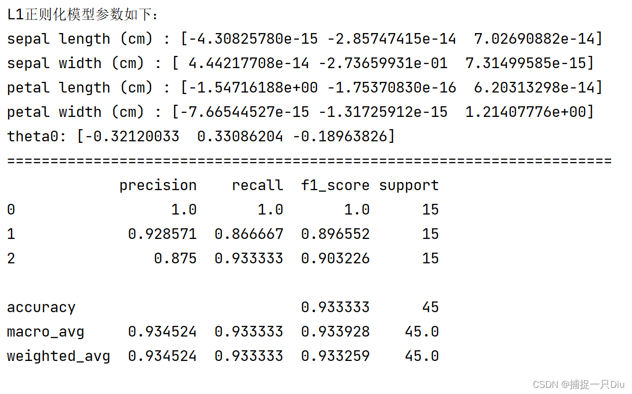
print("L1正则化模型参数如下：")
theta = lg_lr.get_params()
fn = iris.feature_names
for i, w in enumerate(theta[0]):
    print(fn[i], ":", w)
print("theta0:", theta[1])

print("=" * 70)
y_test_prob = lg_lr.predict_prob(X_test)  # 预测概率
y_test_labels = lg_lr.predict(X_test)

plt.figure(figsize=(12, 8))
plt.subplot(221)
lg_lr.plt_loss_curve(lab="L1", is_show=False)

pm = ModelPerformanceMetrics(y_test, y_test_prob)
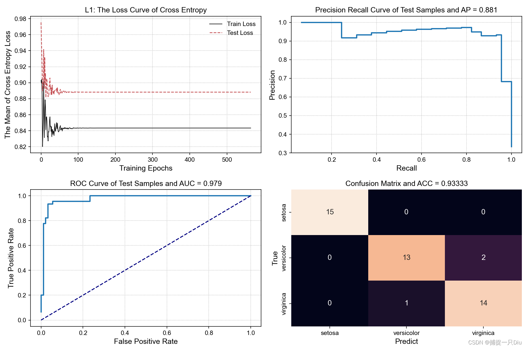
print(pm.cal_classification_report())

pr_values = pm.precision_recall_curve()  # PR指标值
plt.subplot(222)
pm.plt_pr_curve(pr_values, is_show=False)  # PR曲线

roc_values = pm.roc_metrics_curve()  # ROC指标值
plt.subplot(223)
pm.plt_roc_curve(roc_values, is_show=False)  # ROC曲线

plt.subplot(224)
cm = pm.cal_confusion_matrix()
pm.plt_confusion_matrix(cm, label_names=iris.target_names, is_show=False)

plt.tight_layout()
plt.show()