


作者 | 大叔爱学习 编辑 | 汽车人
原文链接:https://www.zhihu.com/question/521494294/answer/3178312617
点击下方卡片,关注“自动驾驶之心”公众号
ADAS巨卷干货,即可获取
本文只做学术分享,如有侵权,联系删文
Swin Transformer的提出,就是让Transformer也有CNN的Block和层级这个多尺度的概念。Vit的作者在Paper的最后面提出,只在Classification方面做了尝试,其他的留给后人。因为在图像的其他下游任务中,比如目标检测,语义分割,图像生成,都需要更细的粒度。那就要调整patch的大小,如果Patch很小,那么计算量就会很大。Swin Transformer的出现,解决了Vit在下游任务表现不好,计算量大等问题,证明了Transformer可以在各类图像任务中战胜CNN。
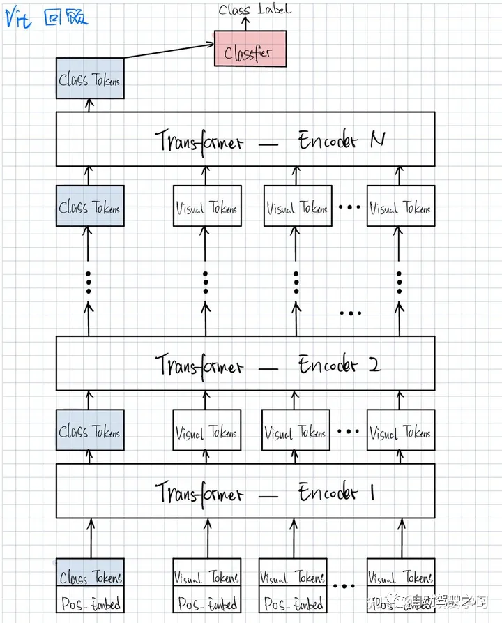
Vit 结构回顾Swin的作者也在开篇强调,将Transformer从NLP转到Image,会有2个挑战。
尺寸问题:比如一张街景图片,里面有车和行人,但车和行人在尺寸上面就非常的不同,这在NLP领域就没有这个问题。
分辨率问题:图像的高分辨率,如果以Pixel作为基本单元,那么每一个Pixel就是一个Token,这个序列的长度对于目前的计算资源来说,高不可攀。所以之前的工作要么是用特征图来当做Transformer的输入,要么就是把图像打成patch(Vit的做法),减少Resolution,要么就是把图片划分成一个个小窗口,在窗口里面做Self-attention(Swin的做法)。所有这些方法,都是为了减少Token序列长度。
Swin Transformer的设计思路
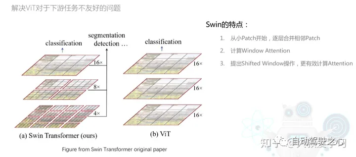
Swin选择的粒度是Window,而不是Patch。从最小的Patch开始,去合并相邻的Patch。另外,在计算Self-Attention的时候,Swin是在Window上计算Attention,而不再是像Vit一样计算Patch的Attention。另外提出的Shift-Window Attention可以更好的提高性能,这个在下一篇再讲。
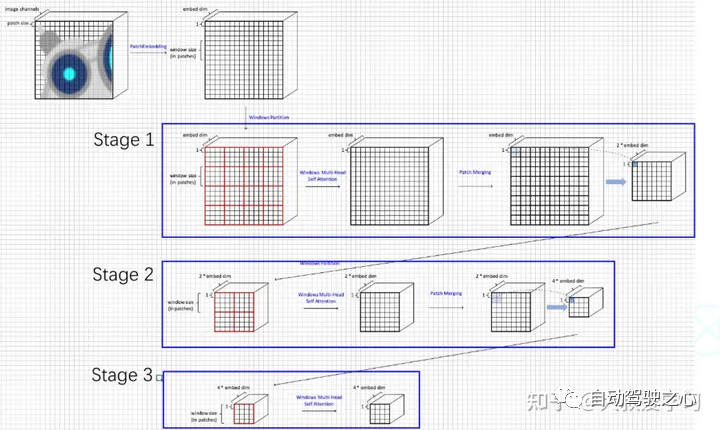
Swin Transformer结构
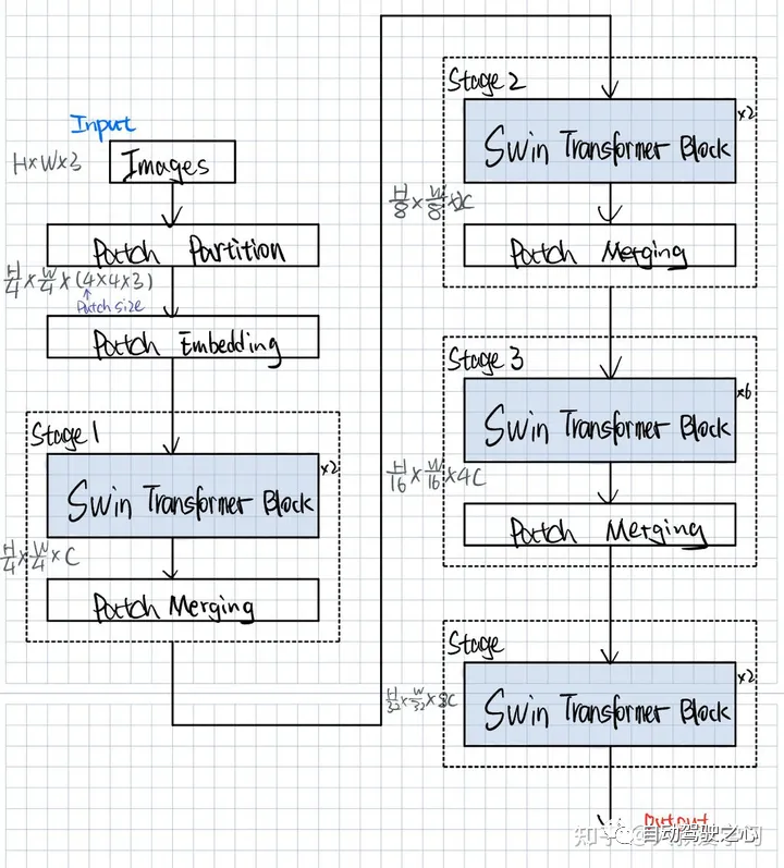
Patch Partition和Patch Embedding就是我们在Vit中说过的先把图像切成块,然后再做一个Projection映射,通常通过Conv2d实现,其实就是对Patch进行特征的提取。得到Patch Embedding后的Visual Token,每一个Visual Token的维度是96维度(可以理解为特征图的channel)。
接着,Swin就分成4个Stages,每个Stage的操作基本上相同。每个Stage里面包含一个Swin Transformer Block和Patch Merging。每一个Swin Transformer Block x2 的意思是由1个W-MSA(Window Multi Self-Attention)和1个SW-MSA(Shifted Window Multi Self-Attention)组成。x6 顾名思义就是3组W-MSA和SW-MSA组成。
Swin Transformer模型结构2:蓝色都是模型的一些网络结构层。立方体表示一个Tensor。Swin对Tensor的大小做了变化。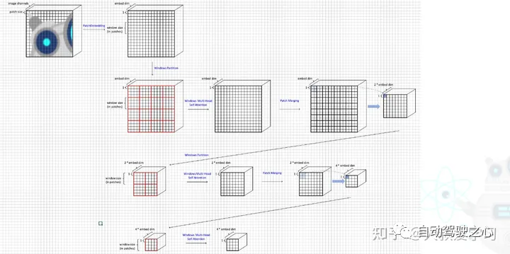
Patch Embedding
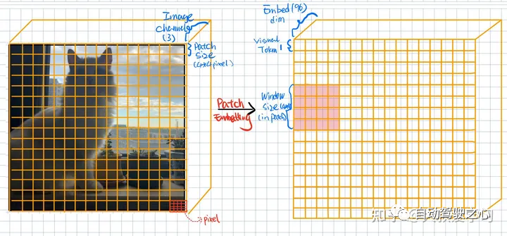
这里Input就是一张彩色猫咪图片,它的Image Channel是3。Patch Size=4,也就表示每一个Patch有4 x 4的Pixel组成。那么Input的Patch个数就是16 x 16。我们会把这些Patch做一个Flatten,然后送入Linear Projection(Conv2d)去进行编码,每一个Patch都会被编码成一个Visual Token,Visual Token的大小就是1 x 1。他的Channel数是embedding编码后的特征维度Embed dim=96。
这些Visual Tokens在Vit中,就会全部送入Encoder中去做Self-Attention,也就是num_token x num_token的Attention计算。但是Swin提出这样的计算量是非常大的,所以它采取的是先将Embedding后的tokens进行Window划分,然后每个Window内部的Visual Tokens去计算在Window内部自己的Attention。可以理解为攘外必先安内。
class PatchEmbedding(nn.Layer):
    def __init__(self, patch_size=4, embed_dim=96):
        super().__init__()
        self.patch_embed = nn.Conv2D(3, embed_dim, kernel_size=patch_size, stride=patch_size)
        self.norm = nn.LayerNorm(embed_dim)

    def forward(self, x):
        x = self.patch_embed(x) # [n, embed_dim, h', w']
        x = x.flatten(2) # [n, embed_dim, h'*w']
        x = x.transpose([0, 2, 1]) #[n, h'*w', embed_dim]
        x = self.norm(x) #[n, num_patches, embed_dim]
        return x
Window Partition
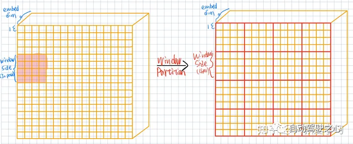
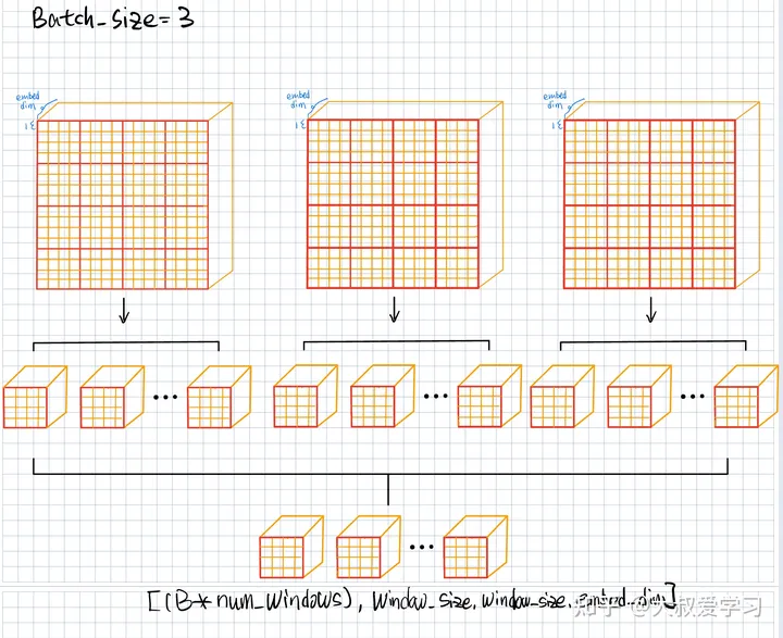
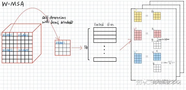
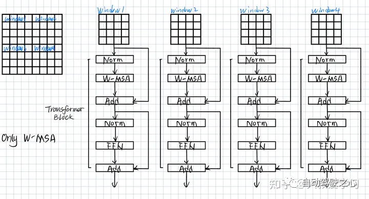
在Patch Embedding后,我们再把Feature切一次,用window的形式切一次(本质上其实和patch一样),这些Windows(4 x 4)没有交叉(Overlap)。
如果是Vit,那么它的做法就是每一个红色小方格和其他红色小方格送到Transformer做Attention。Swin觉得这样计算量比较大,而是使用WMSA (Windows Multi-Head Self Attention)。比如左边的图,左上角第一个红色窗口(4 x 4=16 patches)内部,自己做Self-Attention。和其他window没有关系。每个Window都做自己的。每个Window,输入4 x 4个Tokens,输出也是4 x 4个Tokens。这就是W-MSA。
def windows_partition(x, window_size):
B, H, W, C = x.shape
# B, H/ws, ws, W/ws, ws, C
x = x.reshape([B, H//window_size, window_size, W//window_size, window_size, C])
# B, H/ws, W/ws, ws, ws, c
x = x.transpose([0, 1, 3, 2, 4, 5])
# B * H/ws * W/ws, ws, ws, c
x = x.reshape([-1, window_size, window_size, C])
# x = x.reahspe([-1, window_size*window_size, C]) # [B*num_windows, ws*ws, C]
return x
# CLASS 5
def windows_reverse(windows, window_size, H, W):
# windows: [B*num_windows, ws*ws, C]
B = int(windows.shape[0] // ( H / window_size * W / window_size))
x = windows.reshape([B, H//window_size, W//window_size, window_size, window_size, -1])
x = x.transpose([0, 1, 3, 2, 4, 5]) # [B, H/ws, ws, W/ws, ws, C]
x = x.reshape([B, H, W, -1]) #[B, H, W, C]
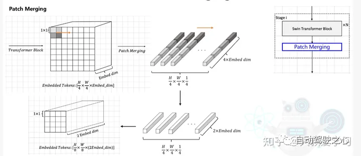
return xPatch Merging
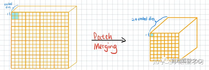
Swin规定,每一次做Patch(或者说Token)融合的时候,就是相邻的4个Patch(Token)做Merging。相邻的4个Patch变成1个,但是它的维度从embed_dim变成了2 x embed_dim。Feature map就变小了。
# CLASS 5
class PatchMerging(nn.Layer):
    def __init__(self, input_resolution, dim):
        super().__init__()
        self.resolution = input_resolution
        self.dim = dim
        self.reduction = nn.Linear(4 * dim, 2 * dim) # projection
        self.norm = nn.LayerNorm(4 * dim)

    def forward(self, x):
        h, w = self.resolution
        b, _, c = x.shape  # [n, num_patches, embed_dim]

        # TODO 1: 得到x的新Shape表示: [B, H, W, C]
        x = x.reshape([b, h, w, c])

        # TODO 2: 为实现Merge, 进行数据拆分, 得到多个数据Shape: [B, H//2, W//2, C]
        x0 = x[:, 0::2, 0::2, :]
        x1 = x[:, 0::2, 1::2, :]
        x2 = x[:, 1::2, ::2, :]
        x3 = x[:, 1::2, 1::2, :]

        # TODO 3: 得到新的x数据:拼接拆分的数据得到Shape: [B, H//2, W//2, 4C]
         x = paddle.concat([x0, x1, x2, x3], axis=-1)

        # TODO 4: 修改x的Shape: [[B, (H//2)*(W//2), 4C]]
        x = x.reshape([b, -1, 4*c])

        # TODO 5: 利用已有的norm和线性层实现最后的Merge映射, 注意这里为PreNorm(先归一化哦)
        x = self.norm(x)

        x = self.reduction(x)
        return x
Stage3全过程
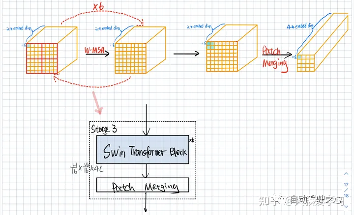
在Stage2,对Patch Merging后的,会进入Stage3,我们继续进行Window的Partition切分(Window Size每次都一样4 x 4),Partition后,我们还在Window内部去做Attention,并不影响其他的窗口。然后再做Patch Merging。Feature Map的Resulotion降低1/2(4 x 4),维度升高(4 x embed dim)。
这里Transformer Block x 6,就是将上面讲的步骤循环了6次,算6次的attention。下面讲讲Swin Transformer Block里面是什么。
Swin Transformer Block
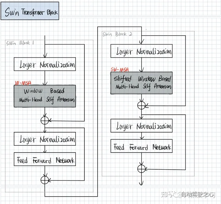
可以看到,每个Block由2部分组成,W-MSA(Window Based Multi-Head Attention)和SW-MSA(Shifted Window Based Multi-Head Attention)。本篇着重讲解左半部分,另一半部分留到下一篇。
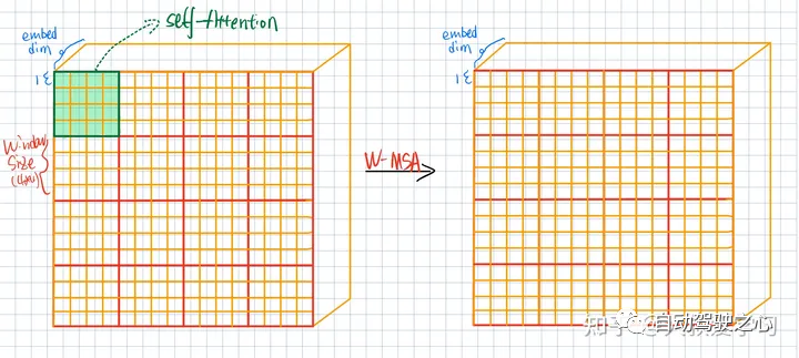
W-MSA(Window Multi-Head Attention)
每个Window里有16个Patches(Tokens)。每个Window分开做Attention,互相不做。
关于为什么MSA的计算量比Swin要大,下面是复杂度的推导。
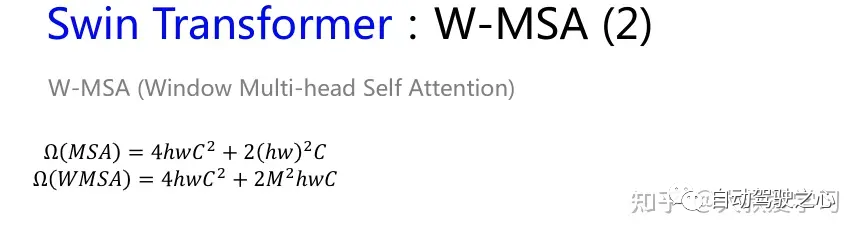
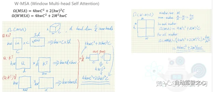
公式本身不重要,重要的是知道Transformer是怎么计算的。
import paddle
import paddle.nn as nn
from mask import generate_mask
paddle.set_device('cpu')

# CLASS 5
class Mlp(nn.Layer):
    def __init__(self, dim, mlp_ratio=4.0, dropout=0.):
        super().__init__()
        self.fc1 = nn.Linear(dim, int(dim * mlp_ratio))
        self.fc2 = nn.Linear(int(dim * mlp_ratio), dim)
        self.act = nn.GELU()
        self.dropout = nn.Dropout(dropout)

    def forward(self, x):
        x = self.fc1(x)
        x = self.act(x)
        x = self.dropout(x)
        x = self.fc2(x)
        x = self.dropout(x)
        return x


class WindowAttention(nn.Layer):
    def __init__(self, dim, window_size, num_heads):
        super().__init__()
        self.dim = dim
        self.dim_head = dim // num_heads
        self.num_heads = num_heads
        self.scale = self.dim_head ** -0.5
        self.softmax = nn.Softmax(axis=-1)
        self.qkv = nn.Linear(dim,
                             dim * 3)
        self.proj = nn.Linear(dim, dim)

        ###### BEGIN Class 6: Relative Position Bias
        self.window_size = window_size
        self.relative_position_bias_table = paddle.create_parameter(
            shape=[(2*window_size-1)*(2*window_size-1), num_heads],
            dtype='float32',
            default_initializer=nn.initializer.TruncatedNormal(std=.02))
        coord_h = paddle.arange(self.window_size)
        coord_w = paddle.arange(self.window_size)
        coords = paddle.stack(paddle.meshgrid([coord_h, coord_w])) #[2, ws, ws]
        coords = coords.flatten(1) #[2, ws*ws]
        relative_coords = coords.unsqueeze(2) - coords.unsqueeze(1)
        relative_coords = relative_coords.transpose([1, 2, 0])
        relative_coords[:, :, 0] += self.window_size - 1
        relative_coords[:, :, 1] += self.window_size - 1

        relative_coords[:, :, 0] *= 2*self.window_size - 1
        relative_coords_index = relative_coords.sum(2)
        print(relative_coords_index)
        self.register_buffer('relative_coords_index', relative_coords_index)
        ###### END Class 6: Relative Position Bias

    ###### BEGIN Class 6: Relative Position Bias
    def get_relative_position_bias_from_index(self):
        table = self.relative_position_bias_table  # [2m-1 * 2m-1, num_heads]
        print('table shape=', table.shape)
        index = self.relative_coords_index.reshape([-1]) # [M^2, M^2] - > [M^2*M^2]
        print('index shape =', index.shape)
        relative_position_bias = paddle.index_select(x=table, index=index) # [M*M, M*M, num_heads]
        return relative_position_bias
    ###### END Class 6: Relative Position Bias

    def transpose_multi_head(self, x):
        new_shape = x.shape[:-1] + [self.num_heads, self.dim_head]
        x = x.reshape(new_shape)
        x = x.transpose([0, 2, 1, 3]) #[B, num_heads, num_patches, dim_head]
        return x

    # CLASS 6
    def forward(self, x, mask=None):
        # x: [B*num_windows, ws*ws, c]
        B, N, C = x.shape
        print('xshape=', x.shape)
        qkv = self.qkv(x).chunk(3, axis=-1)
        q, k, v = map(self.transpose_multi_head, qkv)
        q = q * self.scale
        attn = paddle.matmul(q, k, transpose_y=True)
        # [B*num_windows, num_heads, num_patches, num_patches]  num_patches = windows_size * window_size = M * M

        print('attn shape=', attn.shape)
        ###### BEGIN Class 6: Relative Position Bias
        relative_position_bias = self.get_relative_position_bias_from_index()
        relative_position_bias = relative_position_bias.reshape([self.window_size * self.window_size, self.window_size * self.window_size, -1])
        # [M*M, M*M, num_heads]
        relative_position_bias = relative_position_bias.transpose([2, 0, 1]) #[num_heads, M*M, M*M]
        attn = attn + relative_position_bias.unsqueeze(0)
        ###### END Class 6: Relative Position Bias
        print('attn shape=', attn.shape)

        ###### BEGIN Class 6: Mask
        if mask is None:
            attn = self.softmax(attn)
        else:
            attn = attn.reshape([x.shape[0]//mask.shape[0], mask.shape[0], self.num_heads, mask.shape[1], mask.shape[1]])
            attn = attn + mask.unsqueeze(1).unsqueeze(0)
            attn = attn.reshape([-1, self.num_heads, mask.shape[1], mask.shape[1]])
            attn = self.softmax(attn)
        ###### END Class 6: Mask

        out = paddle.matmul(attn, v)
        out = out.transpose([0, 2, 1, 3])
        out = out.reshape([B, N, C])
        out = self.proj(out)
        return out


# CLASS 5
class SwinBlock(nn.Layer):
    def __init__(self, dim, input_resolution, num_heads, window_size, shift_size=0):
        super().__init__()
        self.dim =dim
        self.resolution = input_resolution
        self.window_size = window_size
        self.shift_size = shift_size

        self.attn_norm = nn.LayerNorm(dim)
        self.attn = WindowAttention(dim, window_size, num_heads)

        self.mlp_norm = nn.LayerNorm(dim)
        self.mlp = Mlp(dim)

        if self.shift_size > 0:
            attn_mask = generate_mask(window_size=self.window_size,
                                      shift_size=self.shift_size,
                                      input_resolution=self.resolution)
        else:
            attn_mask = None
        self.register_buffer('attn_mask', attn_mask)

    def forward(self, x):
        H, W = self.resolution
        B, N, C = x.shape

        h = x
        x = self.attn_norm(x)

        x = x.reshape([B, H, W, C])

        ##### CLASS 6
        if self.shift_size > 0:
            shifted_x = paddle.roll(x, shifts=(-self.shift_size, -self.shift_size), axis=(1, 2))
        else:
            shifted_x = x

        x_windows = windows_partition(shifted_x, self.window_size)
        # [B * num_patches, ws, ws, c]
        x_windows = x_windows.reshape([-1, self.window_size * self.window_size, C])
        attn_windows = self.attn(x_windows, mask=self.attn_mask)
        attn_windows = attn_windows.reshape([-1, self.window_size, self.window_size, C])
        shifted_x = windows_reverse(attn_windows, self.window_size, H, W)

        # reverse cyclic shift
        if self.shift_size > 0:
            x = paddle.roll(shifted_x, shifts=(self.shift_size, self.shift_size), axis=(1, 2))
        else:
            x = shifted_x

        #[B, H, W, C]
        x = x.reshape([B, H*W, C])
        x = h + x

        h = x
        x = self.mlp_norm(x)
        x = self.mlp(x)
        x = h + x
        return x


def main():
    t = paddle.randn((4, 3, 224, 224))
    patch_embedding = PatchEmbedding(patch_size=4, embed_dim=96)
    swin_block_w_msa = SwinBlock(dim=96, input_resolution=[56, 56], num_heads=4, window_size=7, shift_size=0)
    swin_block_sw_msa = SwinBlock(dim=96, input_resolution=[56, 56], num_heads=4, window_size=7, shift_size=7//2)
    patch_merging = PatchMerging(input_resolution=[56, 56], dim=96)

    print('image shape = [4, 3, 224, 224]')
    out = patch_embedding(t) # [4, 56, 56, 96]
    print('patch_embedding out shape = ', out.shape)
    out = swin_block_w_msa(out)
    out = swin_block_sw_msa(out)
    print('swin_block out shape = ', out.shape)
    out = patch_merging(out)
    print('patch_merging out shape = ', out.shape)


if __name__ == "__main__":
    main()
接下来主要讲讲Swin Transformer中最重要的模块:SW-MSA(Shifted Window Multi-head Self Attention)。
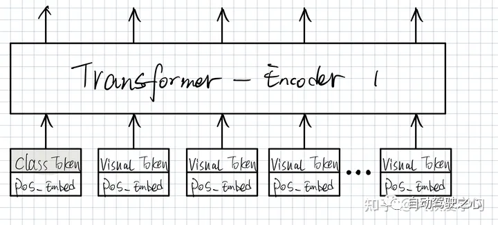
Patch是图像的小块,比如4 x 4的像素。每个Patch最后会变成1,或者Visual Token。它的维度是embed_dim。Visual Tokens(编码后的特征)会进入Tansformer中。Vit,是把所有的Visual Tokens全部拉直,送入Transformer中。
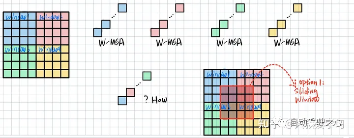
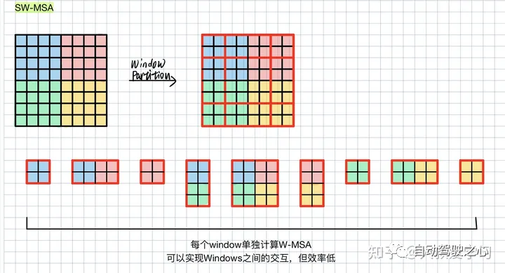
下图最左边每一个小格,对应着上图中的每一个Visual Token(tensor)。Window里是4 x 4的Visual Tokens。Swin是在Window当中单独去做Window Attention。与Vit不同,本Window内的Visual Tokens去算自己内部的attention,这和Vit的Multi-head attention没有本质区别。但这里Windows之间是没有交互的。Window 1中的元素,看不到Window 4的信息。
注意:如果windows之间不交互信息,即window不做Shifted window,可能会有影响。但效果也是可以的。作者做了实验,效果整体来说也是很不错的。
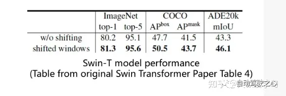
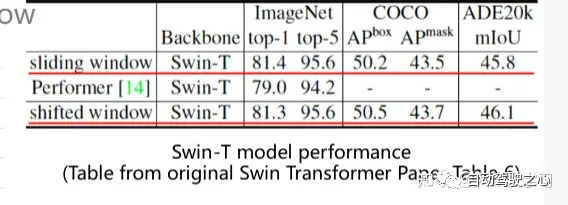
同一个颜色的Window去做Attention,不同颜色之间,目前还没有关系。如果想看全局global信息,我们可以用类似卷积的操作。画一个sliding window去做滑框。这也是可以work的。如图中的论文提到的。但这样计算量比较大,速度比较慢。Swin提出了其他的办法Shifted Window。但我们应该明白,算不同window的关联信息,不只有Swin提供的一种方法。
SW-MSA(Shifted Window Multi-head Self Attention)
那么Swin到底是如何做Shifted Window的呢?
Swin为了让Window之间关联信息,采用了Shifted Window的方法。我们划分了9个大小不同的Windows,对不同大小的Window计算Attention。这样做,某种程度上我们对global信息进行了融合。但是这样方式并不高效,Swin提出了一种Shifted Winodw的概念。
后面大部分篇幅主要是讲述Shifted Winodw如何巧妙地,高效地去计算这9个Window的Attention.
说先讲一个图像位移和循环填充的概念,如下图:
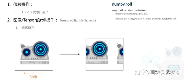
位移操作:1<<3,图像位移更简单
图像/Tensor的roll操作:循环填充
下面看下Swin是怎么做位移和循环填充的:
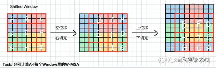
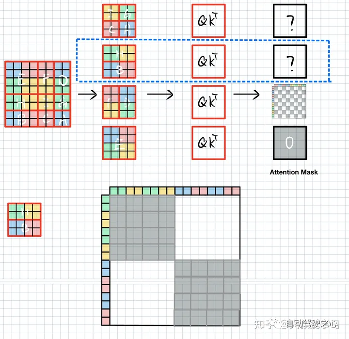
先向左边位移,下边填充,shift的尺寸是window_size/2。然后在往上位移,在下面填充。记住,不论我们怎么做,都是为了更高效地去计算9个不同块的attn。
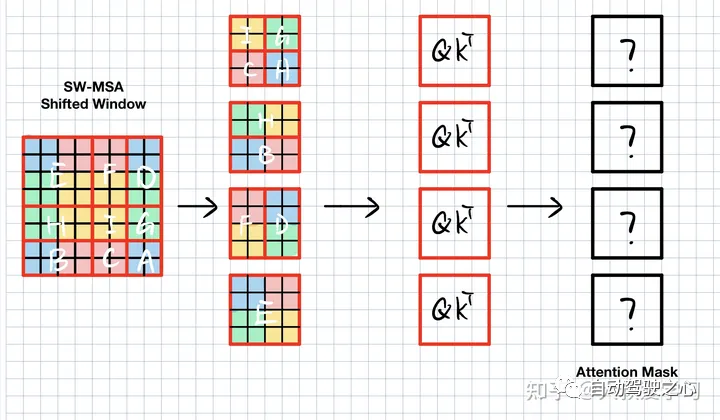
可以看到,这样排布之后,E和W-MSA的window是没有区别的。F和D是切了2块。我们算F的时候,不能算D。H和B同理。IGCA我们只要4个小块。
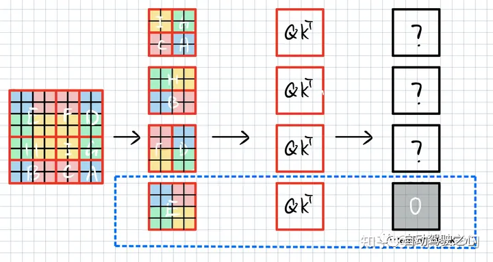
E是M x M的,最下面的方格。把每一个点flatten。所以就是M^2 x M^2。也就是E可以自己做Attention。和Swin1一样,不用动。但是到了F和D,当我们计算F时,我们不希望要右边D的信息(或者mask 0)。这样就达到了只算F的目的。
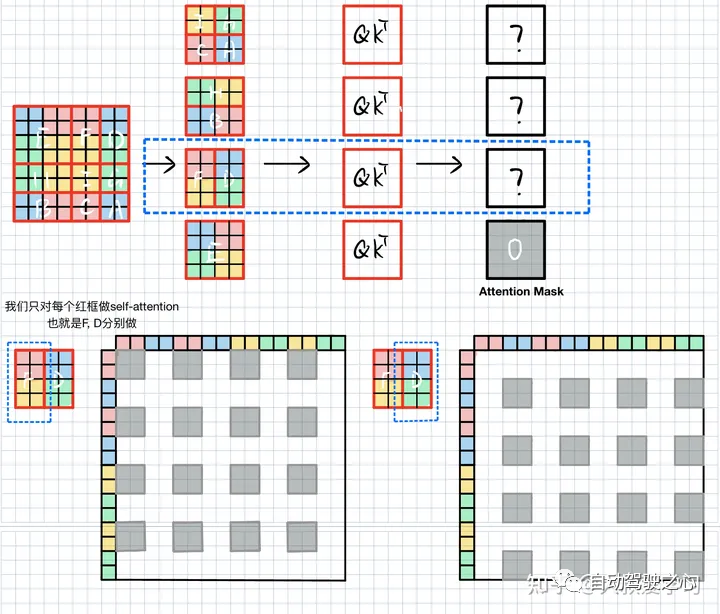
我们可以发现,如果我们只要红黄,阴影部分就是我们要的,其他部分,都是我们不要的。阴影部分填0,其他
同理右边,如下图:我们只要蓝色和绿色,其他不要。
最终关于F和D。如下图所示
同理,H和B如下图所示:
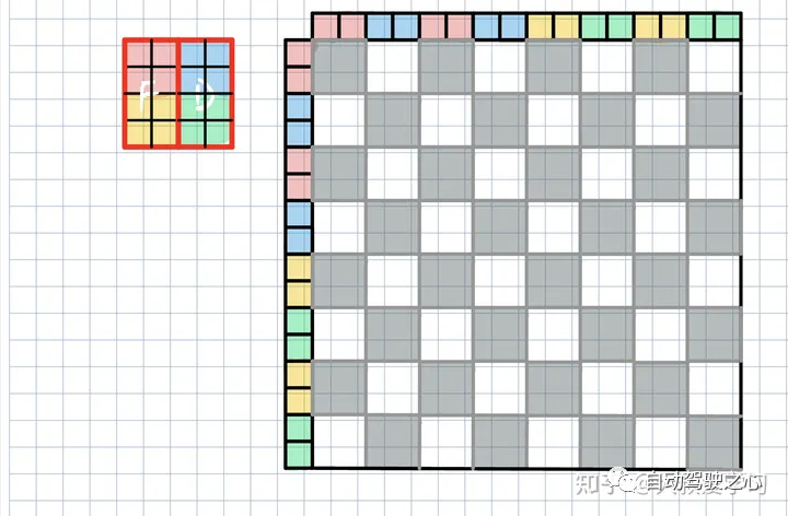
IGCA如下:每个颜色只关心自己颜色。
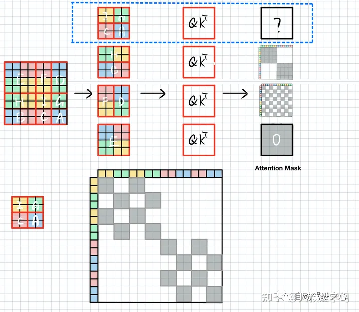
最终SW-MSA+Mask图如下:

阴影部分给的0,不要的给的-100。因为softmax是取exp,exp越小越接近于0。
一定不要忘记,我们上面做的mask,其实也是为了计算9个不同window计算更高效。
文章到这里,Swin Transformer的大体也就介绍完了,和Vit相比,Swin计算更高效,并且可以完成更多的下游任务。Swin的出现,就相当于CNN中的ResNet。可以说是里程碑式的模型。
“百度飞桨:Swin Transformer
”
① 全网独家视频课程
BEV感知、毫米波雷达视觉融合、多传感器标定、多传感器融合、多模态3D目标检测、点云3D目标检测、目标跟踪、Occupancy、cuda与TensorRT模型部署、协同感知、语义分割、自动驾驶仿真、传感器部署、决策规划、轨迹预测等多个方向学习视频(扫码即可学习)
 视频官网:www.zdjszx.com
② 国内首个自动驾驶学习社区
近2000人的交流社区,涉及30+自动驾驶技术栈学习路线,想要了解更多自动驾驶感知(2D检测、分割、2D/3D车道线、BEV感知、3D目标检测、Occupancy、多传感器融合、多传感器标定、目标跟踪、光流估计)、自动驾驶定位建图(SLAM、高精地图、局部在线地图)、自动驾驶规划控制/轨迹预测等领域技术方案、AI模型部署落地实战、行业动态、岗位发布,欢迎扫描下方二维码,加入自动驾驶之心知识星球,这是一个真正有干货的地方,与领域大佬交流入门、学习、工作、跳槽上的各类难题,日常分享论文+代码+视频,期待交流!

③【自动驾驶之心】技术交流群
自动驾驶之心是首个自动驾驶开发者社区,聚焦目标检测、语义分割、全景分割、实例分割、关键点检测、车道线、目标跟踪、3D目标检测、BEV感知、多模态感知、Occupancy、多传感器融合、transformer、大模型、点云处理、端到端自动驾驶、SLAM、光流估计、深度估计、轨迹预测、高精地图、NeRF、规划控制、模型部署落地、自动驾驶仿真测试、产品经理、硬件配置、AI求职交流等方向。扫码添加汽车人助理微信邀请入群,备注:学校/公司+方向+昵称(快速入群方式)

④【自动驾驶之心】平台矩阵,欢迎联系我们!


 1337
1337

 被折叠的 条评论
为什么被折叠?
被折叠的 条评论
为什么被折叠?
 到【灌水乐园】发言


