目标检测Faster-RCNN详解

IT142546355

已于 2022-09-19 07:46:23 修改

阅读量1.2k

点赞数 2

分类专栏：深度学习文章标签： faster-rcnn object detection tensorflow2 目标检测

于 2022-09-19 00:02:43 首次发布

本文链接：https://blog.csdn.net/IT142546355/article/details/126897693

版权

深度学习专栏收录该内容

5 篇文章 0 订阅

订阅专栏

概述

Faster-RCNN是两阶段目标检测算法的典型算法，它不再像古典的目标检测算法使用类似于selective search提取候选框，而是使用RPN(region proposal network)网络提取候选框，因为有RPN网络的加入，Faster-RCNN是可以端对端训练。本文将详解算法结构，正负例划分，损失函数等

代码与环境说明

代码：GitHub - talhuam/faster-rcnn-tf2: A framework for object detection

环境：tensorflow-gpu==2.4.0

显卡：RTX3080 16G

网络架构

backbone

backbone采用的是VGG16，最后一层maxpooling没有做，最终的特征图相较于最初的图片长和宽都缩小了16倍，如果输入图片是600 x 600 x 3，所得的特征图是37 x 37 x 512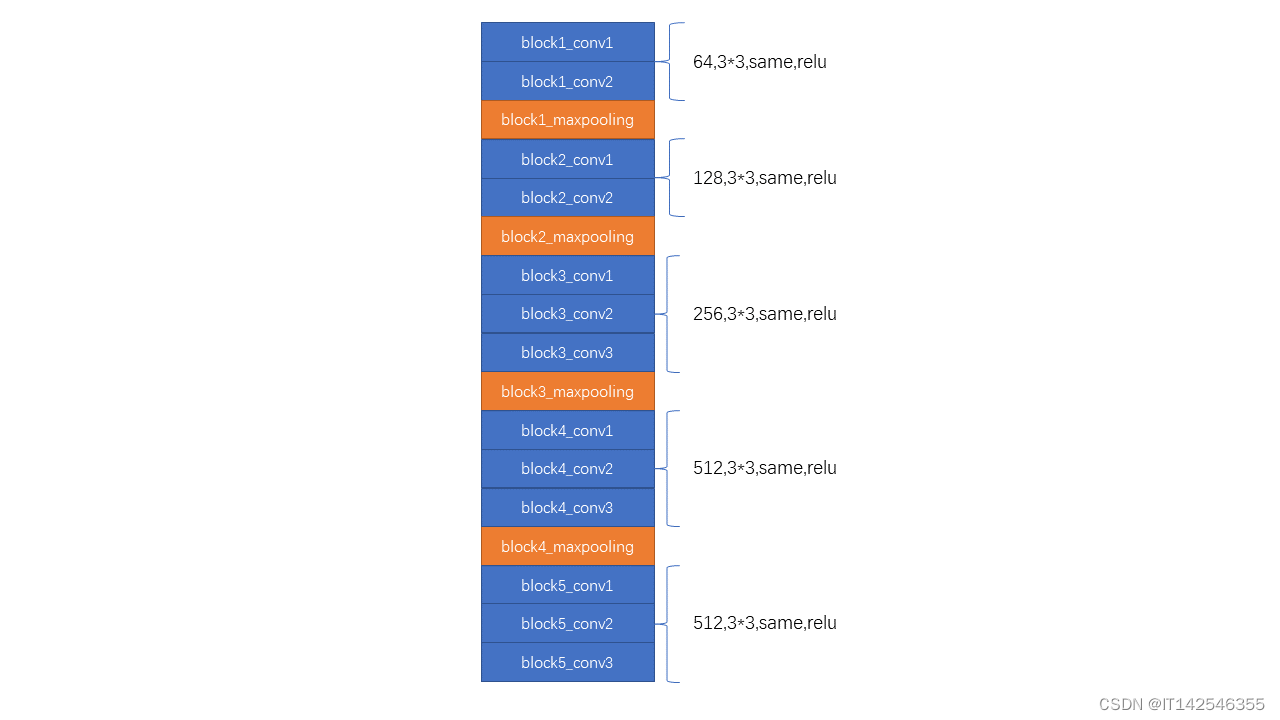

代码实现：

def VGG16(inputs):
    # block1
    x = Conv2D(64, (3, 3), activation='relu', padding='same', name='block1_conv1')(inputs)
    x = Conv2D(64, (3, 3), activation='relu', padding='same', name='block1_conv2')(x)
    x = MaxPooling2D(pool_size=(2, 2), strides=(2, 2), name='block1_pool')(x)

    # block2
    x = Conv2D(128, (3, 3), activation='relu', padding='same', name='block2_conv1')(x)
    x = Conv2D(128, (3, 3), activation='relu', padding='same', name='block2_conv2')(x)
    x = MaxPooling2D(pool_size=(2, 2), strides=(2, 2), name='block2_pool')(x)

    # block3
    x = Conv2D(256, (3, 3), activation='relu', padding='same', name='block3_conv1')(x)
    x = Conv2D(256, (3, 3), activation='relu', padding='same', name='block3_conv2')(x)
    x = Conv2D(256, (3, 3), activation='relu', padding='same', name='block3_conv3')(x)
    x = MaxPooling2D(pool_size=(2, 2), strides=(2, 2), name='block3_pool')(x)

    # block4
    x = Conv2D(512, (3, 3), activation='relu', padding='same', name='block4_conv1')(x)
    x = Conv2D(512, (3, 3), activation='relu', padding='same', name='block4_conv2')(x)
    x = Conv2D(512, (3, 3), activation='relu', padding='same', name='block4_conv3')(x)
    x = MaxPooling2D(pool_size=(2, 2), strides=(2, 2), name='block4_pool')(x)

    # block5
    x = Conv2D(512, (3, 3), activation='relu', padding='same', name='block5_conv1')(x)
    x = Conv2D(512, (3, 3), activation='relu', padding='same', name='block5_conv2')(x)
    x = Conv2D(512, (3, 3), activation='relu', padding='same', name='block5_conv3')(x)
    # x = MaxPooling2D(pool_size=(2, 2), strides=(2, 2), name='block4_pool')

    return x

整体架构

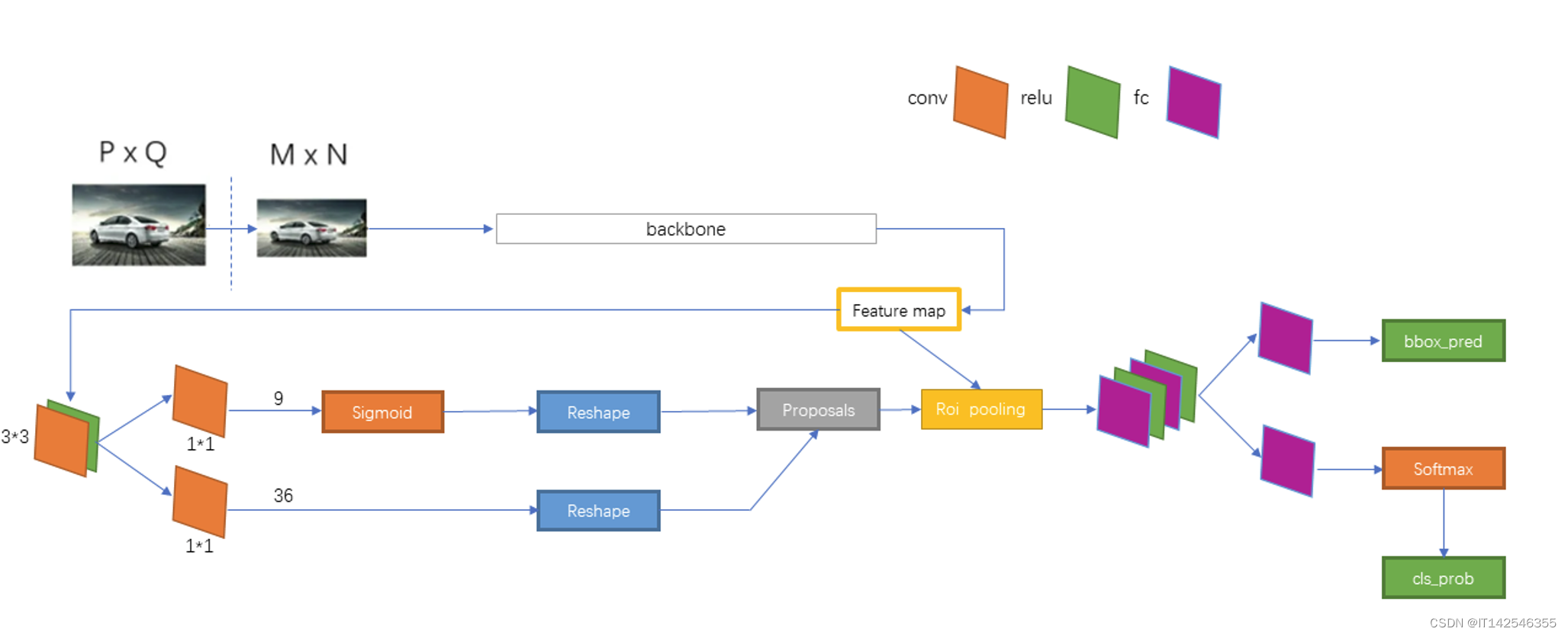
经过vgg16主干网络之后会在经过一次3*3的卷积，此后会分别经过1*1的卷积进行通道降维，两次1*1的卷积如下：

上部分卷积之后会生成(37,37,9)的tensor，9用来预测有物体的概率；
下部分会生成(37,37,9 x 4)的tensor，9*4用来预测框的坐标；

RPN网络之后会进行NMS(non_max_suppression)极大值抑制生成候选框(proposal)。再结合主干网络生成的特征层经过 7 x 7 的ROI pooling层，此过程就是用候选框在特征层上截取，再将截取的部分分成7 x 7的网格，网格内部进行最大池化。截取之前需要将预测出来的 $[t_x,t_y,t_w,t_h]$ 转化为 $[x_{min},y_{min},x_{max},y_{max}]$

最后再将ROI pooling的结果经过全连接层，预测出结果。最后多分类的全连接层用的激活函数是softmax，进行多分类，预测出属于各个类别的概率。回归结果需要将预测出来的 $[t_x,t_y,t_w,t_h]$ 转化为 $[x_{min},y_{min},x_{max},y_{max}]$ 。同类别的框需要再进行一次NMS(阈值0.3)，最终输出结果

正负例划分

RPN正负例

先验框(anchor)的大小有三种，为[128, 256, 512]；三种比例尺寸，为[1:1, 1:2, 2:1]，特征图的每个特征点对应三种大小三种比例共9个先验框。如上所述，如果输入图片的尺寸为600*600，则特征图的尺寸为37*37，那么共有37*37*9=12321个先验框。如下代码会基于特征图的尺寸计算所有先验框的 $[x_{min},y_{min},x_{max},y_{max}]$ 的值并进行归一化

def generate_anchors(sizes=[128, 256, 512], ratios=[[1, 1], [1, 2], [2, 1]]):
    """
    生成基础的9个不同尺寸不同比例的框
    :param sizes:
    :param ratios:
    :return:
    """
    num_anchors = len(sizes) * len(ratios)
    anchors = np.zeros((num_anchors, 4))
    anchors[:, 2:] = np.tile(sizes, [2, len(ratios)]).T

    for i in range(len(ratios)):
        anchors[3 * i:3 * i + 3, 2] = anchors[3 * i:3 * i + 3, 2] * ratios[i][0]
        anchors[3 * i:3 * i + 3, 3] = anchors[3 * i:3 * i + 3, 3] * ratios[i][1]

    anchors[:, 0::2] -= np.tile(anchors[:, 2] * 0.5, [2, 1]).T
    anchors[:, 1::2] -= np.tile(anchors[:, 3] * 0.5, [2, 1]).T
    return anchors


def shift(feature_shape, anchors, stride=16):
    """
    对基础的先验框扩展获得所有的先验框
    :param feature_shape:
    :param anchors:
    :param stride:
    :return:
    """
    shift_x = (np.arange(0, feature_shape[1], dtype=np.float_) + 0.5) * stride
    shift_y = (np.arange(0, feature_shape[0], dtype=np.float_) + 0.5) * stride
    # 框中心点的位置
    shift_x, shift_y = np.meshgrid(shift_x, shift_y)
    # 在一维的shift_x中的元素和shift_y中的元素一一对应形成坐标的x和y
    shift_x = np.reshape(shift_x, (-1))
    shift_y = np.reshape(shift_y, (-1))

    # 将shift_x和shift_y堆叠两次，分别来调整左上角和右下角的坐标
    shifts = np.stack([
        shift_x, shift_y, shift_x, shift_y
    ], axis=0)
    shifts = np.transpose(shifts)
    num_anchors = anchors.shape[0]  # 9

    k = shifts.shape[0]  # 37*37 = 1369
    # 对应维度广播，生成先验框在原图上的左上角和右下角的坐标，shape:[1369(7*7),9,4]
    shifted_anchors = np.reshape(anchors, (1, num_anchors, 4)) + tf.reshape(shifts, (k, 1, 4))
    # (1369 * 9,4)
    shifted_anchors = np.reshape(shifted_anchors, [k * num_anchors, 4])

    return shifted_anchors


def get_anchors(input_shape, sizes=[128, 256, 512], ratios=[[1, 1], [1, 2], [2, 1]], stride=16):
    # ------------------------ #
    # vgg16作为主干特征提取网络，最后一次池化没有做，故而是原有的尺寸的1/16
    # 输入如果是600 * 600,则feature_shape就是37 * 37
    # ------------------------ #
    feature_shape = (int(input_shape[0] / 16), int(input_shape[1] / 16))
    anchors = generate_anchors(sizes, ratios)
    anchors = shift(feature_shape, anchors, stride=stride)
    anchors = anchors.copy()
    # 进行归一化
    anchors[:, 0::2] /= input_shape[1]
    anchors[:, 1::2] /= input_shape[0]
    # 裁剪小于0和大于1的值
    anchors = np.clip(anchors, 0, 1)

    return anchors

所有的先验框和每个真实框(Groud Truth box)计算IoU，IoU大于0.7的作为正例(标签为1)；介于0.3到0.7之间的先验框忽略掉(标签为-1)，不参与计算loss；小于0.3的先验框为负例(标签为0)。其中正例的 $[x_{min},y_{min},x_{max},y_{max}]$ 需要转化为 $[t_x^*,t_y^*,t_w^*,t_h^*]$ ，转化公式如下：

$\begin{aligned} &t_x^*=(x^*-x_a)/w_a & t_y^*=(y^*-y_a)/h_a \\ &t_w^*=log(w^*/w_a) & t_h^*=log(h^*/h_a) \end{aligned}$

代码实现：

# ----------------------------------------------------------------- #
# 将 真实框 和 重合度高的先验框 转化为FRCNN预测结果的格式：[center_x, center_y, width, height]
# ----------------------------------------------------------------- #
# 真实框转化
box_center = 0.5 * (box[2:] + box[:2])
box_wh = box[2:] - box[:2]
# 先验框转化
assigned_anchors_center = 0.5 * (assigned_anchors[:, 2:4] + assigned_anchors[:, :2])
assigned_anchors_wh = assigned_anchors[:, 2:4] - assigned_anchors[:, :2]
# ----------------------------------------------------------------- #
# 计算t_star
# ----------------------------------------------------------------- #
encoded_box[:, :2][assign_mask] = (box_center - assigned_anchors_center) / assigned_anchors_wh
encoded_box[:, :2][assign_mask] /= np.array(variance)[:2]

encoded_box[:, 2:4][assign_mask] = np.log(box_wh/assigned_anchors_wh)
encoded_box[:, 2:4][assign_mask] /= np.array(variance)[2:]

正负例样本数总和256，正负例各128，正例不足用负例填充，超过总数256的标签值置为-1忽略掉，代码实现如下：

# --------------------------------------- #
# 对正样本和负样本进行筛选，训练样本之和为256
# --------------------------------------- #
pos_idx = np.where(classification > 0)[0]
num_pos = len(pos_idx)
if num_pos > self.num_sample // 2:
	num_pos = self.num_sample // 2
	disable_index = np.random.choice(pos_idx, size=(len(pos_idx) - self.num_sample // 2), replace=False)
	classification[disable_index] = -1
	regression[disable_index, -1] = -1

neg_idx = np.where(classification == 0)[0]
num_neg = self.num_sample - num_pos
if len(neg_idx) > num_neg:
	disable_index = np.random.choice(neg_idx, size=(len(neg_idx) - num_neg), replace=False)
	classification[disable_index] = -1
	regression[disable_index, -1] = -1

模型预测正负例

RPN网络正向传播之后，会进行NMS非极大值抑制过滤出k个候选框(proposal)，NMS阈值为0.7。k个候选框将和每个真实框计算IoU，候选框的标签值(cat,dog,...)为对应IoU最大的真实框的标签值，和真实框最大IoU大于等于0.5的作为正例，介于0到0.5之间的作为负例，正例和负例数相加为128，正例不足的用负例填充

# 获得每个建议框roi最对应的真实框的iou
max_iou = np.max(iou, axis=1)  # [len(R) + len(bboxes),] 又 [num_roi,]
gt_assignment = np.argmax(iou, axis=1)  # [num_roi,]

# 和哪个GT的IoU最大，标签就是哪个GT的标签，[num_roi,]
gt_roi_label = label[gt_assignment]

# ------------------------------------------------------------ #
# 和GT的IoU大于pos_iou_thresh是正例
# 将正例控制在n_sample/2之下,如果超过了则随机截取，如果不够则用负例填充
# ------------------------------------------------------------ #
pos_indices = np.where(max_iou >= self.pos_iou_thresh)[0]
pos_roi_per_this_image = int(min(self.n_sample // 2, pos_indices.size))
if pos_indices.size > pos_roi_per_this_image:
	# replace：True可以重复先择,False不可以重复选择，元素不够则报错
	pos_indices = np.random.choice(pos_indices, size=pos_roi_per_this_image, replace=False)

# ------------------------------------------------------------ #
# 和GT的IoU大于neg_iou_thresh_low,小于neg_iou_thresh_high的作为负例
# 正例数量和负例的数量相加等于n_sample
# ------------------------------------------------------------ #
neg_indices = np.where((max_iou >= self.neg_iou_thresh_low) & (max_iou < self.neg_iou_thresh_high))[0]
neg_roi_per_this_image = self.n_sample - pos_roi_per_this_image
if neg_roi_per_this_image > neg_indices.size:
	neg_indices = np.random.choice(neg_indices, size=neg_roi_per_this_image, replace=True)
else:
	neg_indices = np.random.choice(neg_indices, size=neg_roi_per_this_image, replace=False)

# 正例和负例的索引
keep_indices = np.append(pos_indices, neg_indices)
# 保留下来的正负例框,[n_samples, 4]
sample_roi = R[keep_indices]

损失函数

RPN损失

RPN损失包含两部分，一部分是坐标的回归损失，另一部分是二分类损失(有无object)

回归损失

回归损失使用的是smooth L1损失，公式如下，公式中的 $x=\hat{y}-y$ ：

$smooth\_l1\left\{\begin{matrix}0.5*x^2, if&|x|<1 & \\ |x|-0.5&otherwise & \end{matrix}\right.$

实现代码如下：

def rpn_smooth_l1(sigma=1.0):
    """
    rpn smooth l1 损失，只有正例和GT计算损失
    :param sigma:
    :return:
    """
    sigma_squared = sigma ** 2

    def _rpn_smooth_l1(y_true, y_pred):
        # ----------------------- #
        # y_true [batch_size, num_anchors, 4 + 1]
        # y_pred [batch_size, num_anchors, 4]
        # ----------------------- #
        regression = y_pred
        regression_target = y_true[:, :, :-1]
        # ----------------------- #
        # -1是要忽略的，0是背景，1是存在目标
        # ----------------------- #
        anchor_state = y_true[:, :, -1]
        # ----------------------- #
        # 获取正样本
        # ----------------------- #
        indices = tf.where(tf.keras.backend.equal(anchor_state, 1))
        regression = tf.gather_nd(regression, indices)  # 2-D array
        regression_target = tf.gather_nd(regression_target, indices)  # 2-D array
        # ----------------------- #
        # 计算smooth l1损失:
        # 0.5*x^2 if |x|<1
        # |x|-0.5 otherwise
        # ----------------------- #
        regression_diff = regression - regression_target
        x = tf.abs(regression_diff)
        loss_arr = tf.where(x < 1.0 / sigma_squared,
                            0.5 * sigma_squared * tf.pow(x, 2),
                            x - 0.5 / sigma_squared
                            )
        # 将loss全部加起来
        total_loss = tf.reduce_sum(loss_arr)
        # total_loss 除以样本数，计算平均loss
        num_indices = tf.maximum(1., tf.cast(tf.shape(indices)[0], tf.float32))
        avg_loss = total_loss / num_indices
        return avg_loss

    return _rpn_smooth_l1

分类损失

分类损失使用的是二分类的交叉熵损失，实现代码如下：

def rpn_cls_loss():
    """
    rpn只做二分类，是否有object
    二分类交叉熵损失
    :return:
    """

    def _rpn_cls_loss(y_true, y_pred):
        # ----------------------- #
        # y_true [batch_size,num_anchor,1]
        # y_pred [batch_size,num_anchor,1]
        # -1是要忽略的，0是背景，1是存在目标
        # ----------------------- #
        anchor_state = y_true
        # ----------------------- #
        # 获得无需忽略的所有样本
        # ----------------------- #
        indices_for_not_ignore = tf.where(tf.keras.backend.not_equal(anchor_state, -1))
        y_true_no_ignore = tf.gather_nd(y_true, indices_for_not_ignore)  # 1-D array
        y_pred_no_ignore = tf.gather_nd(y_pred, indices_for_not_ignore)  # 1-D array
        # ----------------------- #
        # 计算交叉熵
        # ----------------------- #
        y_true_no_ignore = tf.cast(y_true_no_ignore, dtype=tf.float32)
        y_pred_no_ignore = tf.cast(y_pred_no_ignore, dtype=tf.float32)
        cross_entropy_loss = tf.keras.losses.binary_crossentropy(y_true_no_ignore, y_pred_no_ignore)
        return cross_entropy_loss

    return _rpn_cls_loss

模型预测损失

模型最终的预测损失也有回归损失和分类损失，和RPN分类损失不一样的是，RPN分类是二分类，即是否有物体，最终模型分类损失是多分类，即属于哪一类(cat? dog? car?...)

回归损失

和RPN回归损失一样，这里用的也是smooth L1损失，代码如下：

def classifier_smooth_l1(num_classes, sigma=1.0):
    """
    最后框的回归损失函数
    :param num_classes:
    :param sigma:
    :return:
    """
    sigma_squared = sigma ** 2
    epsilon = 1e-4

    def _classifier_smooth_l1(y_true, y_pred):
        regression = y_pred
        regression_target = y_true[:, :, 4 * num_classes:]

        regression_diff = regression_target - regression
        x = tf.abs(regression_diff)
        loss_arr = tf.where(x < 1 / sigma_squared,
                            0.5 / sigma_squared * tf.pow(x, 2),
                            x - 0.5 / sigma_squared
                            )

        loss = tf.reduce_sum(loss_arr * y_true[:, :, :4 * num_classes]) * 4
        normalizer = tf.keras.backend.sum(epsilon + y_true[:, :, :4 * num_classes])
        loss = loss / normalizer
        return loss
    return _classifier_smooth_l1

分类损失

多分类交叉熵，实现代码如下：

def classifier_cls_loss():
    """
    最后分类的损失函数
    :return:
    """
    def _classifier_cls_loss(y_true, y_pred):
        return tf.keras.losses.categorical_crossentropy(y_true, y_pred)

    return _classifier_cls_loss

IT142546355

关注

2
点赞
踩
1

收藏

觉得还不错? 一键收藏
0
评论
目标检测Faster-RCNN详解

Faster-RCNN是两阶段目标检测算法的典型算法，它不再像古典的目标检测算法使用类似于selective search提取候选框，而是使用RPN(region proposal network)网络提取候选框，因为有RPN网络的加入，Faster-RCNN是可以端对端训练。本文将详解算法结构，正负例划分，损失函数等
复制链接

扫一扫