【图像加密】Logistic混沌+Arnold置乱图像加密解密【含Matlab源码 1281期】

✅博主简介：热爱科研的Matlab仿真开发者，修心和技术同步精进，Matlab项目合作可私信。
🍎个人主页：海神之光
🏆代码获取方式：
海神之光Matlab王者学习之路—代码获取方式
⛳️座右铭：行百里者，半于九十。

更多Matlab仿真内容点击👇
Matlab图像处理（进阶版）
路径规划（Matlab）
神经网络预测与分类（Matlab）
优化求解（Matlab）
语音处理（Matlab）
信号处理（Matlab）
车间调度（Matlab）

⛄一、混沌图像加密与解密简介

混沌系统图像加密解密理论部分参考链接：
基于混沌系统的图像加密算法设计与应用

⛄二、Arnold置乱图像加密解密简介

0 前言
网络已经成为我们传递信息的主要平台, 为我们提供诸多便捷的同时, 也存在一些安全问题, 特别是一些重要信息的传递.如果在信息传递前先对其进行加密, 能够在一定程度上保护所传递的信息.数字图像作为重要的信息资源在人们的生活中发挥着越来越重要的作用[1], 因此, 数字图像的加密是一项值得研究的重要课题.本文介绍的就是一种基于Arnold变换的图像加解密算法。

1 Arnold变换
将N*N图像上的点 (x, y) 通过如下变换转成 (x′, y′) 如式 (1) , 该变换即称为Arnold变换.通过变换公式可发现, 其变换的本质是点的位置的变换, 并且这种变换保证变换前后的点保持一一对应的关系。

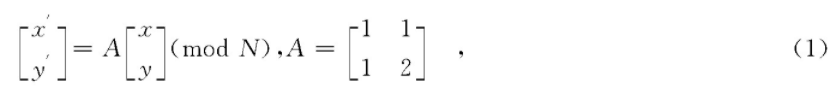
如果将一次变换的输出作为下一次变换的输入, 这就是迭代变换如式 (2) .当一次变换置乱效果不佳时, 往往需要迭代变换获得更好的置乱效果。

2 基于Arnold变换的图像加解密
图像加密也称图像置乱, 是对图像的像素进行混乱和扩散, 使加密后的图像在视觉上无法获得有效信息.空域加密是常用的方法, 分为空域置乱和序列加密.空域置乱是对像素坐标进行变换使其混乱, 解密时恢复原像素坐标.图像的加密既可以作为独立的信息隐藏方法, 也可以用来作为数字水印技术中图像水印的预处理。

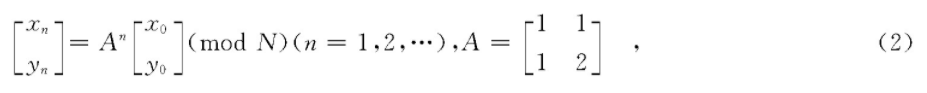
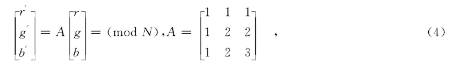
加密图像可以是灰度图像也可以是彩色图像, 如果是灰度图像则需要将各点的灰度值带到新的坐标点, 如果是彩色图像则需要将各点的RGB值带到新的坐标点.本文所加密的图像为彩色图像, 因此首先保存原图点 (x, y) 处的RGB值, 然后使用Arnold变换改变点 (x, y) 位置到 (x′, y′) , 同时将原图点 (x, y) 处的RGB值带到 (x′, y′) 处.我们采用256*256的彩色图像作为原始图像如图1a所示, 在Visual Studio2008平台下运用式 (1) 对原图进行一次Arnold变换, 变换后的效果如图1b所示.

由图1可知, 对图像进行一次Arnold变换后仍会留下较多信息, 故在此基础上继续使用Arnold变换, 通过5次变换后 (见图2b) 其结果在视觉上就很难再获得什么有价值的信息, 在视觉上起到了图像加密的作用.同时变换的次数往往可以作为密钥, 从而在一定程度上提高安全性。

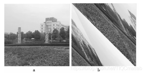
图1 原图和一次Arnold变换结果

图2 第2次和第5次Arnold变换结果
然而此时的加密并不完全可靠, 若已知采用Arnold变换作为加密方式, 则通过暴力求解法, 经过若干次的变换还是可以解密出原图.因此在一般情况下, 我们往往需要在Arnold变换中加入密钥 (ku, kv) , 以提高安全性, 其公式如下:

当需要对图像进行解密时, 则根据加密后的图像中的像素点与原图中的像素点是一一对应的关系进行解密, 因此图像解密的过程为:根据原图中像素点的坐标 (x, y) 按照Arnold变换算出新图中像素点的坐标 (x′, y′) , 获取新像素点 (x′, y′) 的RGB值, 将该值归还给 (x, y) .根据加密过程使用的变换次数, 解密时则要将以上过程重复相应的次数就可以恢复原图 (见图3) 。

3 基于三维Arnold变换的图像加密
前面提到的图像置乱是通过打乱像素点位置而达成目标, 图像的颜色分量值是保持不变的.因此为了提高加密效果, 我们可以在像素点位置已乱的前提下, 再通过改变RGB颜色分量的值对图像进行加密.采用如下三维Arnold变换 (如式4) 进行RGB分量值的改变。

我们将一次Arnold变换后的图像作为原始图像, 在此基础上对各像素点的RGB采用以上公式进行扰乱, 获得如图4所示结果.通过两种加密方式的综合, 则进一步提高了加密图像的安全性.式4中的值可以做相应的改变, 同时可以将变换的次数作为密钥提高安全性。

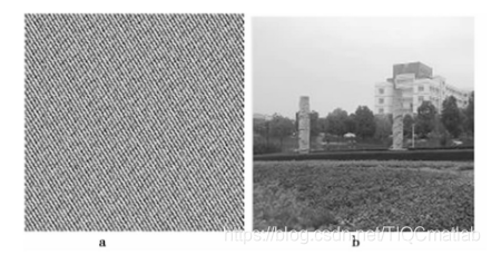
图3 第五次Arnold变换结果, 恢复后的加密图像

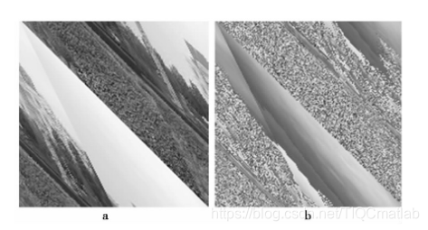
图4 第一次Arnold变换结果, RGB扰乱后的加密图像

⛄三、部分源代码

function jiami
% NOTE:请修改 testImgName，来测试不同输入图像，支持灰度图和 RGB 图
% testImgName = ‘lena’;
% testImgName = ‘lena_color’;
% testImgName = ‘color0’;
% testImgName = ‘lena16x16’;
% testImgName = ‘gray32x32’;
% testImgName = ‘gray2’;
testImgName = ‘pepper_gray’;
% testImgName = ‘1Pixel’;
img = imread(strcat(testImgName, ‘.png’));
[w h rgb] = size(img);
% chaos映射预迭代次数，Logistic映射初始值x0，mu，Arnold置乱次数
Key = [128, 0.7532, 3.8793, 2];

% NOTE:请修改 encryptCount，来测试不同加密次数
% 加密次数
encryptCount = 2;

% 加密
imgEncrypted = img;
for i = 1 : encryptCount
imgEncrypted = encrypt(imgEncrypted, Key);
end

disp(‘###############################’);

% 信息熵计算
if rgb == 3
% 彩色图像
imgR = imgEncrypted(:, :, 1);
imgG = imgEncrypted(:, :, 2);
imgB = imgEncrypted(:, :, 3);
entropyR = informationEntropy(imgR);
entropyG = informationEntropy(imgG);
entropyB = informationEntropy(imgB);
disp(strcat(‘------’, testImgName, ‘,加密次数为:’, num2str(encryptCount), ‘,信息熵 R:’, num2str(entropyR), ‘,G:’, num2str(entropyG), ‘,B:’, num2str(entropyB), ‘------’));
imgR = img(:, :, 1);
imgG = img(:, :, 2);
imgB = img(:, :, 3);
entropyR = informationEntropy(imgR);
entropyG = informationEntropy(imgG);
entropyB = informationEntropy(imgB);
disp(strcat(‘------’, testImgName, ‘,原图信息熵 R:’, num2str(entropyR), ‘,G:’, num2str(entropyG), ‘,B:’, num2str(entropyB), ‘------’));
else
% 灰度图像

% 统计输出
figure;
if rgb == 3
% 彩色图像
subplot(4, 2, 1);
imshow(uint8(img));
title(‘明文’);
subplot(4, 2, 2);
imshow(imgEncrypted);
title(‘密文’);

imgR = img(:, :, 1);
imgG = img(:, :, 2);
imgB = img(:, :, 3);
subplot(4, 2, 3);
imhist(uint8(imgR));
title('明文R分量直方图');
subplot(4, 2, 5);
imhist(uint8(imgG));
title('明文G分量直方图');
subplot(4, 2, 7);
imhist(uint8(imgB));
title('明文B分量直方图');

imgEncryptedR = imgEncrypted(:, :, 1);
imgEncryptedG = imgEncrypted(:, :, 2);
imgEncryptedB = imgEncrypted(:, :, 3);
subplot(4, 2, 4);
imhist(imgEncryptedR);
title('密文R分量直方图');
subplot(4, 2, 6);
imhist(imgEncryptedG);
title('密文G分量直方图');
subplot(4, 2, 8);
imhist(imgEncryptedB);
title('密文B分量直方图');

else
% 灰度图像
subplot(2, 2, 1);
imshow(uint8(img));
title(‘明文’);
subplot(2, 2, 2);
imshow(uint8(imgEncrypted));
title(‘密文’);
subplot(2, 2, 3);
imhist(uint8(img));
title(‘明文直方图’);
subplot(2, 2, 4);
imhist(uint8(imgEncrypted));
title(‘密文直方图’);
end

% 图像受损测试
% 椒盐噪声
delta = 0.02;
imgEncrypted_Noise_Salt = imnoise(imgEncrypted, ‘salt & pepper’, delta);
imgDecrypted_Noise_Salt = imgEncrypted_Noise_Salt;
for i = 1 : encryptCount
imgDecrypted_Noise_Salt = decrypt(imgDecrypted_Noise_Salt, Key);
end
imgDecrypted_Noise_Salt = uint8(imgDecrypted_Noise_Salt);

% 高斯噪声
imgEncrypted_Noise_Gaussian = imnoise(imgEncrypted, ‘gaussian’, delta);
imgDecrypted_Noise_Gaussian = imgEncrypted_Noise_Gaussian;
for i = 1 : encryptCount
imgDecrypted_Noise_Gaussian = decrypt(imgDecrypted_Noise_Gaussian, Key);

% 剪切
imgEncrypted_Croped = crop(imgEncrypted);
imgDecrypted_Croped = imgEncrypted_Croped;
for i = 1 : encryptCount
imgDecrypted_Croped = decrypt(imgDecrypted_Croped, Key);
end
imgDecrypted_Croped = uint8(imgDecrypted_Croped);

figure;
subplot(3, 3, 1);imshow(imgEncrypted);title(‘加密后图像’);
subplot(3, 3, 2);imshow(imgEncrypted_Noise_Salt);title(strcat(‘(1)椒盐噪声ρ=’, num2str(delta)));
subplot(3, 3, 3);imshow(imgDecrypted_Noise_Salt);title(‘(1)解密图像’);
subplot(3, 3, 5);imshow(imgEncrypted_Noise_Gaussian);title(strcat(‘(2)高斯噪声μ=0,σ=’, num2str(delta)));
subplot(3, 3, 6);imshow(imgDecrypted_Noise_Gaussian);title(‘(2)解密图像’);
subplot(3, 3, 8);imshow(imgEncrypted_Croped);title(‘(3)1/16剪切’);
subplot(3, 3, 9);imshow(imgDecrypted_Croped);title(‘(3)解密图像’);

% 明文敏感性

% 彩色图像
gray = imgPlain(w, h, 1);

% bin = dec2bin(gray);
gray = bitxor(gray, 1);
imgPlain(w, h, 1) = gray;
else
% 灰度图像
gray = imgPlain(w, h);
% bin = dec2bin(gray);
gray = bitxor(gray, 1);
imgPlain(w, h) = gray;
end

imgEncrypted1 = imgPlain;
for i = 1 : encryptCount
imgEncrypted1 = encrypt(imgEncrypted1, Key);
end

% 密钥敏感性
Key2 = [128, 0.753200000000001, 3.8793, 1];
imgDecryptedWithKey2 = imgEncrypted;
for i = 1 : encryptCount
imgDecryptedWithKey2 = decrypt(imgDecryptedWithKey2, Key2);
end
figure;
title(strcat(num2str(encryptCount), ‘轮加密’));
subplot(2, 2, 1);
imshow(img);title(‘明文’);
subplot(2, 2, 2);
imshow(imgEncrypted);title(‘密文’);
subplot(2, 2, 3);
imshow(imgDecrypted);title(‘原始密钥的解密结果’);
subplot(2, 2, 4);
imshow(imgDecryptedWithKey2);title(‘密钥改变一位的解密结果’);

disp(strcat(‘------’, testImgName, ‘,加密次数为:’, num2str(encryptCount), ‘,密钥敏感性分析------’));
NPCR(imgEncrypted, imgEncrypted2, ‘密钥改变1个值’);
UACI(imgEncrypted, imgEncrypted2, ‘密钥改变1个值’);

% 相关性
relationType = 2;
relationCount = 1024;
if rgb == 3
% 彩色图像

imgEncryptedR = imgEncrypted(:, :, 1);
imgEncryptedG = imgEncrypted(:, :, 2);
imgEncryptedB = imgEncrypted(:, :, 3);

imgRrelation = relation(imgR, relationType, relationCount, strcat('------', testImgName, ',明文R分量'));
imgGrelation = relation(imgG, relationType, relationCount, strcat('------', testImgName, ',明文G分量'));
imgBrelation = relation(imgB, relationType, relationCount, strcat('------', testImgName, ',明文B分量'));
imgEncryptedRrelation = relation(imgEncryptedR, relationType, relationCount, strcat('------', testImgName, ',密文R分量'));
imgEncryptedGrelation = relation(imgEncryptedG, relationType, relationCount, st
subplot(2, 3, 1);
plot(imgRrelation(1, :), imgRrelation(2, :), '.');
axis([0 256 0 256]);
title('明文R分量灰度值水平相关性');
subplot(2, 3, 2);
plot(imgGrelation(1, :), imgGrelation(2, :), '.');
axis([0 256 0 256]);
title('明文G分量');
subplot(2, 3, 3);
plot(imgBrelation(1, :), imgBrelation(2, :), '.');
axis([0 256 0 256]);
title('明文B分量');

subplot(2, 3, 4);
plot(imgEncryptedRrelation(1, :), imgEncryptedRrelation(2, :), '.');
axis([0 256 0 256]);
title('密文R分量灰度值水平相关性');
subplot(2, 3, 5);
plot(imgEncryptedGrelation(1, :), imgEncryptedGrelation(2, :), '.');
axis([0 256 0 256]);
title('密文G分量');
subplot(2, 3, 6);
plot(imgEncryptedBrelation(1, :), imgEncryptedBrelation(2, :), '.');
axis([0 256 0 256]);
title('密文B分量');    

else
% 灰度图像

figure;
subplot(2, 1, 1);
plot(imgrelation(1, :), imgrelation(2, :), '.');
axis([0 256 0 256]);
title('明文灰度值水平相关性');xlabel('位置(i,j)的像素灰度值');ylabel('位置(i+1,j)的像素灰度值');
subplot(2, 1, 2);
plot(imgEncryptedrelation(1, :), imgEncryptedrelation(2, :), '.');
axis([0 256 0 256]);
title('密文灰度值水平相关性');xlabel('位置(i,j)的像素灰度值');ylabel('位置(i+1,j)的像素灰度值');

end

end

% 加密图像img，Key为密钥矩阵
function imgEncrypted = encrypt(img, Key)
img = double(img);
[w h rgb] = size(img);

if rgb == 3
% 彩色图像

else
% 灰度图像
% % 灰度值替换
% img = logisticReplace(img, Key(3), Key(2), Key(1));
%
% 三维置乱
lengthImg = w * h;
L = floor(lengthImg ^ (1 / 3));
lengthCube = L ^ 3;
img = reshape(img, lengthImg, 1);
Cube1 = reshape(img(1 : lengthCube), L, L, L);
Cube1 = triplePermution(Cube1);

% 变换到二维图像
imgEncrypted(1 : lengthCube, 1) = reshape(Cube1, lengthCube, 1);
imgEncrypted(lengthCube + 1 : lengthImg, 1) = img(lengthCube + 1 : lengthImg, 1);
imgEncrypted = reshape(imgEncrypted, w, h);

% Arnold置乱
imgEncrypted = arnoldPermution(imgEncrypted, Key(4));

end
imgEncrypted = uint8(imgEncrypted);
end

% 加密图像img，Key为密钥矩阵
function imgDecrypted = decrypt(img, Key)
img = double(img);
[w h rgb] = size(img);

if rgb == 3
% 彩色图像

else
% 灰度图像
% Arnold逆置乱
img = arnoldDePermution(img, Key(4));
%
% 三维逆置乱
lengthImg = w * h;
L = floor(lengthImg ^ (1 / 3));
lengthCube = L ^ 3;
img = reshape(img, lengthImg, 1);
Cube1 = reshape(img(1 : lengthCube), L, L, L);
Cube1 = tripleDePermution(Cube1);

% 变换到二维图像
imgDecrypted(1 : lengthCube, 1) = reshape(Cube1, lengthCube, 1);
imgDecrypted(lengthCube + 1 : lengthImg, 1) = img(lengthCube + 1 : lengthImg, 1);
imgDecrypted = reshape(imgDecrypted, w, h);

% % 灰度值替换
% imgDecrypted = logisticDeReplace(imgDecrypted, Key(3), Key(2), Key(1));
end
imgDecrypted = uint8(imgDecrypted);
end

⛄四、运行结果

⛄五、matlab版本及参考文献

1 matlab版本
2014a

2 参考文献
[1]邢顺来,李志斌,周华成.基于Arnold变换和混沌映射的图像加密方法[J].山东广播电视大学学报. 2012,(01)

3 备注
简介此部分摘自互联网，仅供参考，若侵权，联系删除

🍅 仿真咨询
1 各类智能优化算法改进及应用
生产调度、经济调度、装配线调度、充电优化、车间调度、发车优化、水库调度、三维装箱、物流选址、货位优化、公交排班优化、充电桩布局优化、车间布局优化、集装箱船配载优化、水泵组合优化、解医疗资源分配优化、设施布局优化、可视域基站和无人机选址优化

2 机器学习和深度学习方面
卷积神经网络（CNN）、LSTM、支持向量机（SVM）、最小二乘支持向量机（LSSVM）、极限学习机（ELM）、核极限学习机（KELM）、BP、RBF、宽度学习、DBN、RF、RBF、DELM、XGBOOST、TCN实现风电预测、光伏预测、电池寿命预测、辐射源识别、交通流预测、负荷预测、股价预测、PM2.5浓度预测、电池健康状态预测、水体光学参数反演、NLOS信号识别、地铁停车精准预测、变压器故障诊断

3 图像处理方面
图像识别、图像分割、图像检测、图像隐藏、图像配准、图像拼接、图像融合、图像增强、图像压缩感知

4 路径规划方面
旅行商问题（TSP）、车辆路径问题（VRP、MVRP、CVRP、VRPTW等）、无人机三维路径规划、无人机协同、无人机编队、机器人路径规划、栅格地图路径规划、多式联运运输问题、车辆协同无人机路径规划、天线线性阵列分布优化、车间布局优化

5 无人机应用方面
无人机路径规划、无人机控制、无人机编队、无人机协同、无人机任务分配

6 无线传感器定位及布局方面
传感器部署优化、通信协议优化、路由优化、目标定位优化、Dv-Hop定位优化、Leach协议优化、WSN覆盖优化、组播优化、RSSI定位优化

7 信号处理方面
信号识别、信号加密、信号去噪、信号增强、雷达信号处理、信号水印嵌入提取、肌电信号、脑电信号、信号配时优化

8 电力系统方面
微电网优化、无功优化、配电网重构、储能配置

9 元胞自动机方面
交通流 人群疏散 病毒扩散 晶体生长

10 雷达方面
卡尔曼滤波跟踪、航迹关联、航迹融合