


本次要分享的论文是
A
t
t
e
n
t
i
o
n
−
o
v
e
r
−
A
t
t
e
n
t
i
o
n
N
e
u
r
a
l
N
e
t
w
o
r
k
s
f
o
r
R
e
a
d
i
n
g
C
o
m
p
r
e
h
e
n
s
i
o
n
Attention-over-Attention\ Neural\ Networks\ for\ Reading\ Comprehension
Attention−over−Attention Neural Networks for Reading Comprehension,论文链接AoA,论文源自
A
C
L
2017
ACL2017
ACL2017,参考的实现代码代码链接。
好了,老规矩,带着代码看论文。
整体网络结构

任务描述
本篇论文的应用场景是在完形填空的任务上:
<
D
,
Q
,
A
>
<D, Q, A>
<D,Q,A>
其中
D
D
D 是文档,也可以理解为文章,
Q
Q
Q 表示一个询问,也就是
q
u
e
r
y
query
query,
A
A
A 就是我们需要得出的
a
n
s
w
e
r
answer
answer,***
a
n
s
w
e
r
answer
answer 为一个单词,并且该单词在
D
D
D 中出现过。***
任务很简单,其实个人感觉也可以视为一个 Q A QA QA 任务。
模型描述
contextual Embedding
将 D , Q D, Q D,Q 中的每个词经过 w o r d _ e m b e d i n g word\_embeding word_embeding,这里需要注意 D , Q D, Q D,Q 的 E m b e d d i n g Embedding Embedding 矩阵是相同的,也即是所谓的 s h a r e _ e m b e d d i n g share\_embedding share_embedding,那么这样做有什么好处呢?显然,这样做的话, D , Q D, Q D,Q 都能参与 e m b e d d i n g embedding embedding 矩阵的学习, e m b e d d i n g embedding embedding 矩阵也能学习的更好。
然后,将经过 w o r d _ e m b e d d i n g word\_embedding word_embedding 后的 D , Q D, Q D,Q 作为输入,喂给双向的 G R U GRU GRU,然后将双向 G R U GRU GRU 的前向和后向输出做个 c o n c a t concat concat 操作,生成一个 o u t p u t output output,具体公式如下:
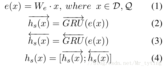
D , Q D, Q D,Q 分别经过这一步操作以后,分别生成 h d o c , h q u e r y h_{doc}, h_{query} hdoc,hquery,其 s h a p e shape shape 分别为 [ ∣ D ∣ ∗ 2 d i m ] , [ ∣ Q ∣ ∗ 2 d i m ] [|D|*2dim], [|Q|*2dim] [∣D∣∗2dim],[∣Q∣∗2dim]。
这一步代码如何实现呢?
  embedding = tf.get_variable('embedding',
    ┆   ┆   ┆ [FLAGS.vocab_size, FLAGS.embedding_size],
    ┆   ┆   ┆ initializer=tf.random_uniform_initializer(minval=-0.05, maxval=0.05))

  regularizer = tf.nn.l2_loss(embedding)

  doc_emb = tf.nn.dropout(tf.nn.embedding_lookup(embedding, documents), FLAGS.dropout_keep_prob)
  doc_emb.set_shape([None, None, FLAGS.embedding_size])

  query_emb = tf.nn.dropout(tf.nn.embedding_lookup(embedding, query), FLAGS.dropout_keep_prob)
  query_emb.set_shape([None, None, FLAGS.embedding_size])

  with tf.variable_scope('document', initializer=orthogonal_initializer()):
    fwd_cell = tf.contrib.rnn.GRUCell(FLAGS.hidden_size)
    back_cell = tf.contrib.rnn.GRUCell(FLAGS.hidden_size)

    doc_len = tf.reduce_sum(doc_mask, reduction_indices=1)
    h, _ = tf.nn.bidirectional_dynamic_rnn(
    ┆   fwd_cell, back_cell, doc_emb, sequence_length=tf.to_int64(doc_len), dtype=tf.float32)
    #h_doc = tf.nn.dropout(tf.concat(2, h), FLAGS.dropout_keep_prob)
    h_doc = tf.concat(h, 2)

  with tf.variable_scope('query', initializer=orthogonal_initializer()):
    fwd_cell = tf.contrib.rnn.GRUCell(FLAGS.hidden_size)
    back_cell = tf.contrib.rnn.GRUCell(FLAGS.hidden_size)

    query_len = tf.reduce_sum(query_mask, reduction_indices=1)
    h, _ = tf.nn.bidirectional_dynamic_rnn(
    ┆   fwd_cell, back_cell, query_emb, sequence_length=tf.to_int64(query_len), dtype=tf.float32)
    #h_query = tf.nn.dropout(tf.concat(2, h), FLAGS.dropout_keep_prob)
    h_query = tf.concat(h, 2)
pair-wise Matching Score
论文中提到,我们可以根据上面生成的 h d o c , h q u e r y h_{doc}, h_{query} hdoc,hquery 来计算两向量的匹配程度。
M
(
i
,
j
)
=
h
d
o
c
(
i
)
T
⋅
h
q
u
e
r
y
(
j
)
M(i, j) = h_{doc}(i)^T\cdot h_{query}(j)
M(i,j)=hdoc(i)T⋅hquery(j)
得到的
M
M
M 矩阵的
s
h
a
p
e
shape
shape 为
[
∣
D
∣
∗
∣
Q
]
∣
[|D|*|Q]|
[∣D∣∗∣Q]∣
实现代码:
M = tf.matmul(h_doc, h_query, adjoint_b=True)
M_mask = tf.to_float(tf.matmul(tf.expand_dims(doc_mask, -1), tf.expand_dims(query_mask, 1)))
Individual Attentions
在上一步中,我们得到一个 M M M 矩阵,由此,可以对该矩阵的每一列做个 s o f t m a x softmax softmax 操作,而每列是由 D D D 行组成,所以论文中称这种操作为 d o c u m e n t − l e v e l a t t e n t i o n document-level\ attention document−level attention。每一列可理解为只考虑了一个 q u e r y _ w o r d query\_word query_word。
α
(
t
)
=
s
o
f
t
m
a
x
(
M
(
1
,
t
)
,
.
.
.
,
M
(
∣
D
∣
,
t
)
)
\alpha (t)=softmax(M(1, t),...,M(|D|, t))
α(t)=softmax(M(1,t),...,M(∣D∣,t))
α
=
[
α
(
1
)
,
α
(
2
)
,
.
.
.
,
α
(
∣
Q
∣
)
]
\alpha = [\alpha (1),\alpha (2),...,\alpha (|Q|)]
α=[α(1),α(2),...,α(∣Q∣)]
###Attention-over-Attention
上面我们做了
d
o
c
u
m
e
n
t
−
l
e
v
e
l
a
t
t
e
n
t
i
o
n
document-level\ attention
document−level attention 操作,同理也可以做
q
u
e
r
y
−
l
e
v
e
l
a
t
t
e
n
t
i
o
n
query-level\ attention
query−level attention 操作:
β
(
t
)
=
s
o
f
t
m
a
x
(
M
(
t
,
1
)
,
.
.
.
,
M
(
t
,
∣
Q
∣
)
)
\beta (t)=softmax(M(t, 1),...,M(t, |Q|))
β(t)=softmax(M(t,1),...,M(t,∣Q∣))
β
=
[
β
(
1
)
,
β
(
2
)
,
.
.
.
,
β
(
∣
D
∣
)
]
\beta = [\beta (1),\beta (2),...,\beta (|D|)]
β=[β(1),β(2),...,β(∣D∣)]
实现代码:
# Softmax over axis
def softmax(target, axis, mask, epsilon=1e-12, name=None):
  with tf.op_scope([target], name, 'softmax'):
    max_axis = tf.reduce_max(target, axis, keep_dims=True)
    target_exp = tf.exp(target-max_axis) * mask
    normalize = tf.reduce_sum(target_exp, axis, keep_dims=True)
    softmax = target_exp / (normalize + epsilon)
    return softmax

alpha = softmax(M, 1, M_mask)##mask矩阵,非零位置为1,反正为0,axis=0为batch
beta = softmax(M, 2, M_mask)
需要注意的是,我看过一些基于 a t t e n t i o n attention attention 方法的论文,大部分都做了类似 d o c u m e n t − l e v e l a t t e n t i o n document-level\ attention document−level attention 操作,这篇论文不仅做了 d o c u m e n t − l e v e l a t t e n t i o n document-level\ attention document−level attention ,还做了 q u e r y − l e v e l a t t e n t i o n query-level\ attention query−level attention,的确是比较有创新的地方。
论文里还对
β
\beta
β 做了简单的处理:
β
=
1
n
∑
t
=
1
∣
D
∣
β
(
t
)
\beta=\frac{1}{n}\sum_{t=1}^{|D|}\beta(t)
β=n1t=1∑∣D∣β(t)
然后做了矩阵乘积操作:
s
=
α
T
β
s=\alpha^T\beta
s=αTβ
如何解释这个矩阵操作呢?直观上看,就像把每个 q u e r y query query 的 w o r d word word去衡量每个 d o c u m e n t − l e v e l document-level document−level 的权重,由此学习出 d o c u m e n t document document 中哪个词更有可能为 a n s w e r answer answer。
实现代码:
query_importance = tf.expand_dims(tf.reduce_mean(beta, 1) / tf.to_float(tf.expand_dims(doc_len, -1)), -1)

s = tf.squeeze(tf.matmul(alpha, query_importance), [2])
###预测部分
上面我们可以得到一个
s
s
s 向量,这个
s
s
s 向量和
d
o
c
u
m
e
n
t
document
document 长度相等,因此若某个词在
d
o
c
u
m
e
n
t
document
document 出现多次,则该词也应该在
s
s
s 中出现多次,该词的概率应该等于其在
s
s
s 出现的概率之和。
p
(
w
∣
D
,
Q
)
=
∑
i
∈
I
(
w
,
D
)
s
i
,
w
∈
V
p(w| D, Q)=\sum_{i\in I(w,D)}^{}s_i,w\in V
p(w∣D,Q)=i∈I(w,D)∑si,w∈V
这部分代码:
unpacked_s = zip(tf.unstack(s, FLAGS.batch_size), tf.unstack(documents, FLAGS.batch_size))

y_hat = tf.stack([tf.unsorted_segment_sum(attentions, sentence_ids, FLAGS.vocab_size) for (attentions, sentence_ids) in unpacked_s])##注意这里面y_hat也就是上面所讲的s向量,但是其经过unsorted_segment_sum操作后,其长度变为vocab_size.
那在
t
r
a
i
n
train
train 时,
o
b
j
e
c
t
_
f
u
n
c
t
i
o
n
object\_function
object_function 具体是怎样呢?
L
=
∑
i
l
o
g
(
p
(
x
)
)
,
x
∈
A
L =\sum_{i}log(p(x)),x\in A
L=i∑log(p(x)),x∈A
实现代码:
下面代码中的一波操作不太好理解,其在
n
l
p
nlp
nlp 代码中很常见,值得好好琢磨。
index = tf.range(0, FLAGS.batch_size) * FLAGS.vocab_size + tf.to_int32(answer)##这里面为啥乘以vocab_size,看下面解释

flat = tf.reshape(y_hat, [-1])## 注意每个样本的y_hat长度为vocab_size,直接将batch_size个flat reshape成一维。
relevant = tf.gather(flat, index)##以index为准,找到flat中对应的值,也就是answer中的词在s向量中的概率值。

loss = -tf.reduce_mean(tf.log(relevant))

accuracy = tf.reduce_mean(tf.to_float(tf.equal(tf.argmax(y_hat, 1), answer)))
个人感想
好了,这篇论文所介绍的网络结构已经介绍完毕了,来谈谈我个人读完这篇论文和代码后的感想。
- 我看过一些 Q A 、 Q G QA、QG QA、QG 等方面的论文,感觉大部分都做了类似论文所说的 d o c u m e n t − l e v e l a t t e n t i o n document-level\ attention document−level attention 操作,也就是结合 q u e r y query query 去 a t t e n t i o n d o c u m e n t attention\ document attention document, 这篇创新的也做了 q u e r y − l e v e l a t t e n t i o n query-level\ attention query−level attention 操作。
- 感觉这篇论文实际上做了两层 a t t e n t i o n attention attention,在第一层中不仅做了 d o c u m e n t − l e v e l a t t e n t i o n document-level\ attention document−level attention ,也做了 q u e r y − l e v e l a t t e n t i o n query-level\ attention query−level attention,第二层中,把结合 q u e r y − l e v e l a t t e n t i o n query-level\ attention query−level attention 的信息对 d o c u m e n t − l e v e l a t t e n t i o n document-level\ attention document−level attention 又做了 a t t e n t i o n attention attention 操作。


 9404
9404


 被折叠的 条评论
为什么被折叠?
被折叠的 条评论
为什么被折叠?
 到【灌水乐园】发言


