万字长文教你从零实现百万参数LLM训练

最新推荐文章于 2025-05-14 15:14:05 发布

Python_金钱豹

最新推荐文章于 2025-05-14 15:14:05 发布

阅读量427

点赞数 8

文章标签：算法人工智能 transformer 数码相机深度学习

本文链接：https://blog.csdn.net/Python_cocola/article/details/147949514

版权

01.引言

制作自己的大型语言模型（LLM）是一件很酷的事情，谷歌、Twitter 和 Facebook 等许多大公司都在这样做。他们会发布不同版本的模型，如 70 亿、130 亿或 700 亿。即使是较小的社区也在这样做。你可能读过关于创建自己的 LLM 的博客或看过相关视频，但它们通常只谈理论，对实际步骤和代码涉及不多。

在这篇文章中，我们将尝试制作一个只有 230 万个参数的 LLM，有趣的是，我们不需要特别多的 GPU。我们将以 LLaMA 1 论文方法为指导。别担心，我们会保持简单并使用一个基本数据集，这样你就能看到创建自己的百万参数 LLM 有多么容易。

闲话少说，我们直接开始吧！

02.了解LLama结构

在使用 LLaMA 方法创建我们自己的 LLM 之前，有必要了解一下 LLaMA 的架构。下面是原始Transformer结构和 LLaMA结构的对比图。

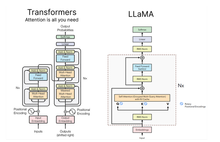
以下我们来逐章节介绍一下 LLaMA 结构中的改进点。

03.使用RMSNorm进行前归一化

在 LLaMA 结构中，采用了一种名为 RMSNorm 的技术，对每个Transformer子层的输入进行归一化处理。这种方法受到 GPT-3 的启发，旨在优化与LayerNorm相关的计算成本。RMSNorm 的性能与 LayerNorm 相似，但运行时间大大缩短（7%∼64%）。

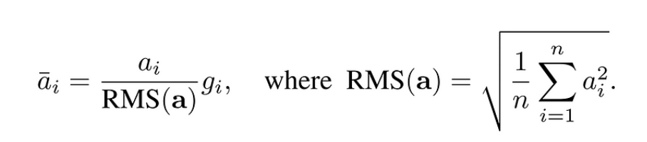
为此，RMSNorm强调重新缩放不变性，并根据均方根（RMS）统计量调节输入总和。其主要动机是通过去除均方根统计量来简化 LayerNorm。

04.采用SwiGLU激活函数

LLaMA 从 PaLM结构中汲取灵感，引入了 SwiGLU 激活函数。要理解 SwiGLU，首先必须掌握 Swish 激活函数。SwiGLU 对 Swish 进行了扩展，包括一个带有密集网络的自定义层，用于对输入激活进行拆分和乘法运算。

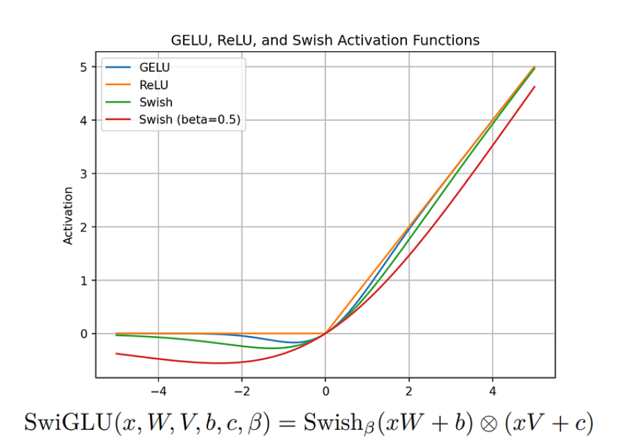
其目的是通过引入更复杂的激活函数来增强模型的表现力。有关 SwiGLU 的更多详情，请参阅相关论文。

论文链接：https://arxiv.org/pdf/2002.05202v1

05.采用RoPE位置编码

旋转位置编码RoPE 是 LLaMA 中使用的一种位置嵌入。它使用旋转矩阵对绝对位置信息进行编码，并在自注意公式中自然地包含明确的相对位置依赖性。RoPE 具有多种优势，例如可扩展到各种序列长度，并且随着相对距离的增加，Token间的依赖性会逐渐减弱。

这是通过与旋转矩阵相乘对相对位置进行编码来实现的，从而产生衰减的相对距离–这是自然语言编码的理想特性。对数学细节感兴趣的人可以参阅 RoPE 论文。

论文：https://arxiv.org/pdf/2104.09864v4

除这些概念外，LLaMA 论文还介绍了其他重要方法，包括使用带有特定参数的 AdamW 优化器、高效实现（如 xformers 库中的因果多头注意力算子），以及手动实现Transformer层的后向传播函数，以优化后向传播过程中的计算。

06.导入基本库

在简单介绍了基本理论后，我们接着来编写代码，首先导入我们的基本依赖库：

# PyTorch for implementing LLM (No GPU)import torch# Neural network modules and functions from PyTorchfrom torch import nnfrom torch.nn import functional as F# NumPy for numerical operationsimport numpy as np# Matplotlib for plotting Loss etc.from matplotlib import pyplot as plt# Time module for tracking execution timeimport time# Pandas for data manipulation and analysisimport pandas as pd# urllib for handling URL requests (Downloading Dataset)import urllib.request

此外，我们创建一个存储模型参数配置的字典对象。

# Configuration object for model parametersMASTER_CONFIG = {    # Adding parameters later}

这种方法保持了灵活性，允许在未来根据需要添加更多参数配置。

07.下载数据集

在最初的 LLaMA 论文中，他们采用了多种开源数据集来训练和评估模型。

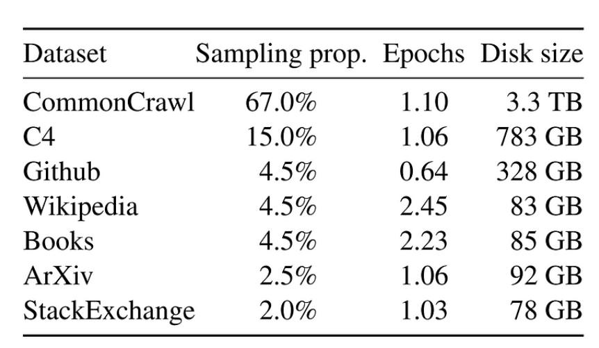
遗憾的是，对于小型项目来说，利用大量数据集可能并不现实。因此，在我们的实施过程中，我们将采取一种更为温和的方法，创建一个大幅缩减的 LLaMA 版本。

考虑到无法获取海量数据的限制，我们将重点使用 TinyShakespeare 数据集训练简化版的 LLaMA。

链接：https://github.com/karpathy/char-rnn/blob/master/data/tinyshakespeare/input.txt

该开源数据集可在上述链接获取，包含约 40,000 行来自莎士比亚各种作品的文本。

LLaMA 是在一个包含 1.4 万亿个字符的庞大数据集上进行训练的，而我们的数据集 TinyShakespeare 包含约 100 万个字符。首先，让我们下载数据集：

# The URL of the raw text file on GitHuburl = "https://raw.githubusercontent.com/karpathy/char-rnn/master/data/tinyshakespeare/input.txt"
# The file name for local storagefile_name = "tinyshakespeare.txt"
# Execute the downloadurllib.request.urlretrieve(url, file_name)

该 Python 脚本从指定的 URL 获取 tinyshakespeare 数据集，并以文件名 "tinyshakespeare.txt "保存到本地。

接下来，让我们确定词汇量的大小，它代表了数据集中唯一的字符数。下面是统计代码片段：

# Read the content of the datasetlines = open("tinyshakespeare.txt", 'r').read()# Create a sorted list of unique characters in the datasetvocab = sorted(list(set(lines)))
# Display the first 10 characters in the vocabulary listprint('Printing the first 10 characters of the vocab list:', vocab[:10])# Output the total number of characters in our dataset (Vocabulary Size)print('Total number of characters in our dataset (Vocabulary Size):', len(vocab))

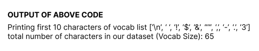
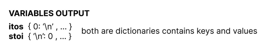
接着，我们要在整数到字符 (itos) 和字符到整数 (stoi) 之间创建映射。代码如下：

# Mapping integers to characters (itos)itos = {i: ch for i, ch in enumerate(vocab)}# Mapping characters to integers (stoi)stoi = {ch: i for i, ch in enumerate(vocab)}

08.定义编解码函数

在最初的 LLaMA 论文中，使用了谷歌的 SentencePiece 字节对编码Tokenizer。不过，为了简单起见，我们将选择基本的字符级Tokenizer。让我们创建编码和解码函数，随后将其应用于我们的数据集：

# Encode function: Converts a string to a list of integers using the mapping stoidef encode(s):    return [stoi[ch] for ch in s]# Decode function: Converts a list of integers back to a string using the mapping itosdef decode(l):    return ''.join([itos[i] for i in l])# Example: Encode the string "hello" and then decode the resultdecode(encode("morning"))

最后一行将输出单词moning，以确认编码函数和解码函数的正常运行。

现在，我们将数据集转换为 torch 张量，指定其数据类型，以便使用 PyTorch 进行进一步操作：

# Convert the dataset into a torch tensor with specified data type (dtype)dataset = torch.tensor(encode(lines), dtype=torch.int8)# Display the shape of the resulting tensorprint(dataset.shape)

输出结果 torch.Size([1115394])显示，我们的数据集包含约一百万个Tokens。值得注意的是，这比包含 1.4 万亿个Tokens的 LLaMA 数据集要小得多。

09.拆分数据集

接着，我们将创建一个函数，负责将数据集拆分为训练集、验证集或测试集。在机器学习或深度学习项目中，这种拆分对于开发和评估模型至关重要，同样的原则也适用于大型语言模型（LLM）的训练过程：

# Function to get batches for training, validation, or testingdef get_batches(data, split, batch_size, context_window, config=MASTER_CONFIG):    # Split the dataset into training, validation, and test sets    train = data[:int(.8 * len(data))]    val = data[int(.8 * len(data)): int(.9 * len(data))]    test = data[int(.9 * len(data)):]    # Determine which split to use    batch_data = train    if split == 'val':        batch_data = val    if split == 'test':        batch_data = test    # Pick random starting points within the data    ix = torch.randint(0, batch_data.size(0) - context_window - 1, (batch_size,))    # Create input sequences (x) and corresponding target sequences (y)    x = torch.stack([batch_data[i:i+context_window] for i in ix]).long()    y = torch.stack([batch_data[i+1:i+context_window+1] for i in ix]).long()    return x, y

既然我们已经定义了切分函数，那么让我们来确定两个对这一过程至关重要的参数：

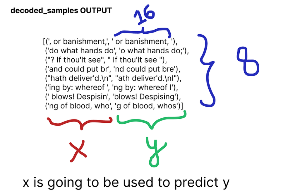
# Update the MASTER_CONFIG with batch_size and context_window parametersMASTER_CONFIG.update({    'batch_size': 8,          # Number of batches to be processed at each random split    'context_window': 16      # Number of characters in each input (x) and target (y) sequence of each batch})

batch_size 决定每次随机切分处理多少个批次，而 context_window 则指定每个批次的每个输入 (x) 和目标 (y) 序列中的字符数。

让我们以数据集的第 8 个批次和上下文窗口为16的训练集中打印一个随机样本：

# Obtain batches for training using the specified batch size and context windowxs, ys = get_batches(dataset, 'train', MASTER_CONFIG['batch_size'], MASTER_CONFIG['context_window'])# Decode the sequences to obtain the corresponding text representationsdecoded_samples = [(decode(xs[i].tolist()), decode(ys[i].tolist())) for i in range(len(xs))]# Print the random sampleprint(decoded_samples)

结果如下：

10.评估策略

现在，我们将创建一个函数，专门用于评估我们自创的 LLaMA 架构。之所以要在定义实际模型方法之前这样做，是为了在训练过程中进行持续评估。

@torch.no_grad()  # Don't compute gradients for this functiondef evaluate_loss(model, config=MASTER_CONFIG):    # Placeholder for the evaluation results    out = {}
    # Set the model to evaluation mode    model.eval()    # Iterate through training and validation splits    for split in ["train", "val"]:        # Placeholder for individual losses        losses = []        # Generate 10 batches for evaluation        for _ in range(10):            # Get input sequences (xb) and target sequences (yb)            xb, yb = get_batches(dataset, split, config['batch_size'], config['context_window'])
            # Perform model inference and calculate the loss            _, loss = model(xb, yb)
            # Append the loss to the list            losses.append(loss.item())        # Calculate the mean loss for the split and store it in the output dictionary        out[split] = np.mean(losses)
    # Set the model back to training mode    model.train()
    return out

在训练迭代过程中，我们使用损失作为评估模型性能的指标。我们的函数迭代训练和验证集，计算每次拆分 10 次的平均损失，最后返回结果。然后使用 model.train() 将模型设置回训练模式。

11.建立基础神经网络

首先我们来构建一个基本的神经网络，稍后将利用 LLaMA 技术对其进行改进。

# Definition of a basic neural network classclass SimpleBrokenModel(nn.Module):    def __init__(self, config=MASTER_CONFIG):        super().__init__()        self.config = config        # Embedding layer to convert character indices to vectors (vocab size: 65)        self.embedding = nn.Embedding(config['vocab_size'], config['d_model'])        # Linear layers for modeling relationships between features        # (to be updated with SwiGLU activation function as in LLaMA)        self.linear = nn.Sequential(            nn.Linear(config['d_model'], config['d_model']),            nn.ReLU(),  # Currently using ReLU, will be replaced with SwiGLU as in LLaMA            nn.Linear(config['d_model'], config['vocab_size']),        )        # Print the total number of model parameters        print("Model parameters:", sum([m.numel() for m in self.parameters()]))

在当前的架构中，嵌入层的词汇量为 65 个，代表了我们数据集中的字符数目。由于这是我们的基础模型，我们在线性层中使用 ReLU 作为激活函数；不过，稍后将用 LLaMA 中使用的 SwiGLU 代替。

要为基础模型创建前向传递，我们必须在 NN 模型中定义一个forward函数。

# Definition of a basic neural network classclass SimpleBrokenModel(nn.Module):    def __init__(self, config=MASTER_CONFIG):        # Rest of the code                ...         # Forward pass function for the base model        def forward(self, idx, targets=None):            # Embedding layer converts character indices to vectors            x = self.embedding(idx)
            # Linear layers for modeling relationships between features            a = self.linear(x)
            # Apply softmax activation to obtain probability distribution            logits = F.softmax(a, dim=-1)            # If targets are provided, calculate and return the cross-entropy loss            if targets is not None:                # Reshape logits and targets for cross-entropy calculation                loss = F.cross_entropy(logits.view(-1, self.config['vocab_size']), targets.view(-1))                return logits, loss            # If targets are not provided, return the logits            else:                return logits        # Print the total number of model parameters        print("Model parameters:", sum([m.numel() for m in self.parameters()]))

这个前向传递函数将字符索引（idx）作为输入，应用嵌入层，将结果传递给线性层，应用 softmax 激活以获得概率分布（logits）。如果提供了目标，它会计算交叉熵损失，并同时返回 logits 和损失。如果没有提供目标，则只返回预测logits。

要实例化该模型，我们可以直接调用该类，并打印 "简单神经网络模型 "中的参数总数。我们将线性层的维数设置为 128，并在配置对象中指定了这一数值：

# Update MASTER_CONFIG with the dimension of linear layers (128)MASTER_CONFIG.update({    'd_model': 128,})# Instantiate the SimpleBrokenModel using the updated MASTER_CONFIGmodel = SimpleBrokenModel(MASTER_CONFIG)# Print the total number of parameters in the modelprint("Total number of parameters in the Simple Neural Network Model:", sum([m.numel() for m in model.parameters()]))

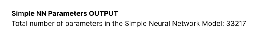
可以看到，我们的简单神经网络模型包含约 33,000 个参数。

12.训练基础神经网络

在定义了基本的神经网络结构后，为了计算损失，我们只需将拆分后的数据集输入模型即可：

# Obtain batches for training using the specified batch size and context windowxs, ys = get_batches(dataset, 'train', MASTER_CONFIG['batch_size'], MASTER_CONFIG['context_window'])# Calculate logits and loss using the modellogits, loss = model(xs, ys)

为了训练该基础模型并记录其性能，我们需要指定一些参数。我们总共要训练 1000 个epoch。将batchsize从 8 增加到 32，并将 log_interval 设置为 10，表示代码将每 10 个批次打印或记录一次训练进度信息。在优化方面，我们将使用 Adam 优化器。

# Update MASTER_CONFIG with training parametersMASTER_CONFIG.update({    'epochs': 1000,          # Number of training epochs    'log_interval': 10,      # Log information every 10 batches during training    'batch_size': 32,        # Increase batch size to 32})# Instantiate the SimpleBrokenModel with updated configurationmodel = SimpleBrokenModel(MASTER_CONFIG)# Define the Adam optimizer for model parametersoptimizer = torch.optim.Adam(    model.parameters(),      # Pass the model parameters to the optimizer)

让我们执行训练过程，记录该基础模型的损失，包括参数总数。此外，为清晰起见，每一行都有注释：

# Function to perform trainingdef train(model, optimizer, scheduler=None, config=MASTER_CONFIG, print_logs=False):    # Placeholder for storing losses    losses = []
    # Start tracking time    start_time = time.time()    # Iterate through epochs    for epoch in range(config['epochs']):        # Zero out gradients        optimizer.zero_grad()        # Obtain batches for training        xs, ys = get_batches(dataset, 'train', config['batch_size'], config['context_window'])        # Forward pass through the model to calculate logits and loss        logits, loss = model(xs, targets=ys)        # Backward pass and optimization step        loss.backward()        optimizer.step()        # If a learning rate scheduler is provided, adjust the learning rate        if scheduler:            scheduler.step()        # Log progress every specified interval        if epoch % config['log_interval'] == 0:            # Calculate batch time            batch_time = time.time() - start_time
            # Evaluate loss on validation set            x = evaluate_loss(model)
            # Store the validation loss            losses += [x]
            # Print progress logs if specified            if print_logs:                print(f"Epoch {epoch} | val loss {x['val']:.3f} | Time {batch_time:.3f} | ETA in seconds {batch_time * (config['epochs'] - epoch)/config['log_interval'] :.3f}")
            # Reset the timer            start_time = time.time()            # Print learning rate if a scheduler is provided            if scheduler:                print("lr: ", scheduler.get_lr())    # Print the final validation loss    print("Validation loss: ", losses[-1]['val'])
    # Plot the training and validation loss curves    return pd.DataFrame(losses).plot()# Execute the training processtrain(model, optimizer)

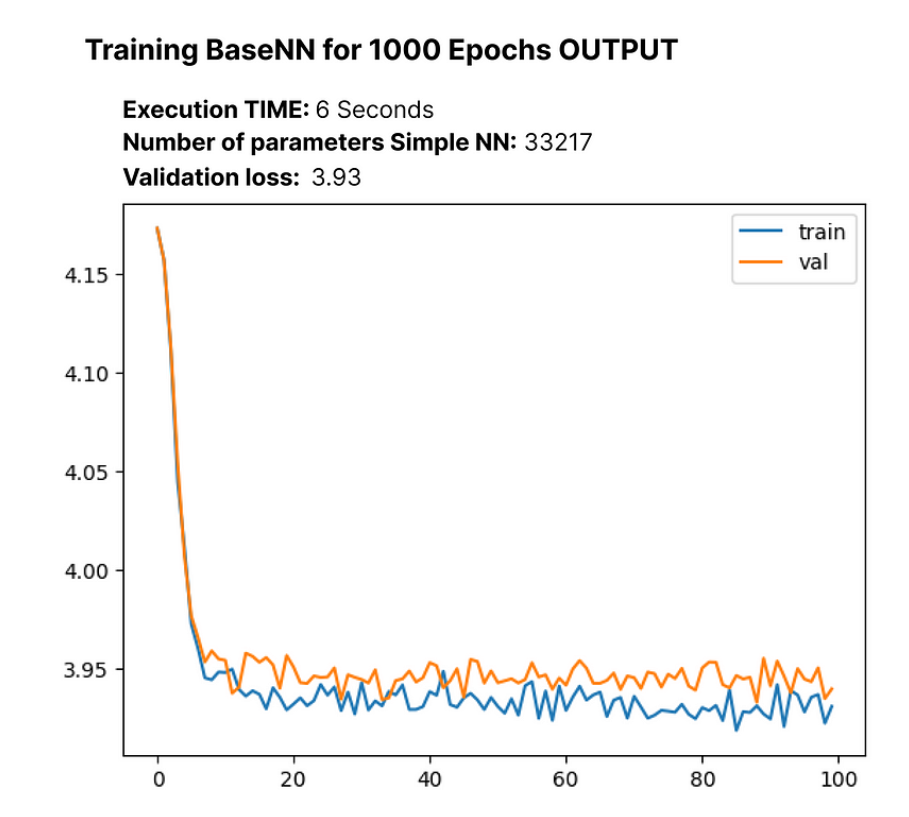
训练前的初始交叉熵损失为 4.17，100 个epoch后基本收敛降至 3.93。

我们的基础模型在logits 后面加入了一个 softmax 层，将数字向量转换为概率分布。此外，我们在使用内置的 F.cross_entropy 函数时可以直接输入非规范化的 logits。因此，我们将对模型进行相应修改。

# Modified SimpleModel class without softmax layerclass SimpleModel(nn.Module):    def __init__(self, config):
       # Rest of the code       ...    def forward(self, idx, targets=None):        # Embedding layer converts character indices to vectors        x = self.embedding(idx)
        # Linear layers for modeling relationships between features        logits = self.linear(x)        # If targets are provided, calculate and return the cross-entropy loss        if targets is not None:            # Rest of the code            ...

让我们重新创建更新后的 SimpleModel，并对其进行 1000个 epoch训练，以观察其变化：

# Create the updated SimpleModelmodel = SimpleModel(MASTER_CONFIG)# Obtain batches for trainingxs, ys = get_batches(dataset, 'train', MASTER_CONFIG['batch_size'], MASTER_CONFIG['context_window'])# Calculate logits and loss using the modellogits, loss = model(xs, ys)# Define the Adam optimizer for model parametersoptimizer = torch.optim.Adam(model.parameters())# Train the model for 100 epochstrain(model, optimizer)

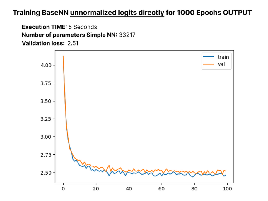
100个epoch后将损失减小到 2.51 后，让我们来探索一下拥有约 33,000 个参数的语言模型如何在推理过程中生成文本。我们将创建一个 "generate "函数，代码如下：

# Generate function for text generation using the trained modeldef generate(model, config=MASTER_CONFIG, max_new_tokens=30):    idx = torch.zeros(5, 1).long()    for _ in range(max_new_tokens):        # Call the model        logits = model(idx[:, -config['context_window']:])        last_time_step_logits = logits[            :, -1, :        ]  # all the batches (1), last time step, all the logits        p = F.softmax(last_time_step_logits, dim=-1)  # softmax to get probabilities        idx_next = torch.multinomial(            p, num_samples=1        )  # sample from the distribution to get the next token        idx = torch.cat([idx, idx_next], dim=-1)  # append to the sequence    return [decode(x) for x in idx.tolist()]# Generate text using the trained modelgenerate(model)

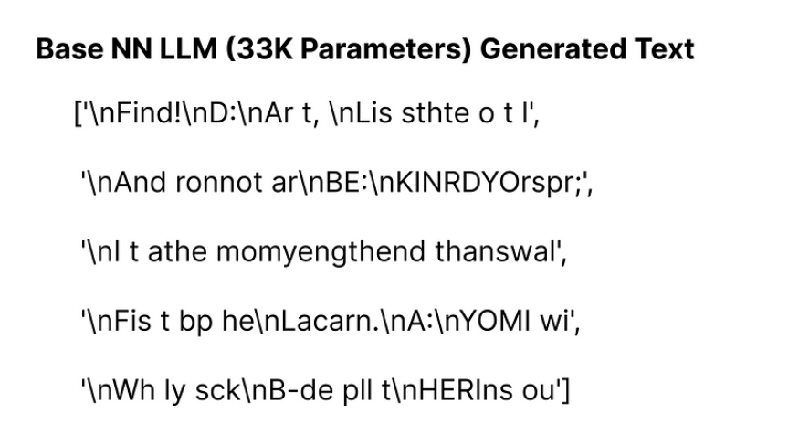
我们的基本模型大约有 33K 个参数，生成的文本看起来并不出色。不过，既然我们已经为这个简单的模型奠定了基础，下一节我们将继续构建 LLaMA 架构。

13.复现LLama结构

在本文的前半部分，我们介绍了基本概念，现在，我们将把这些概念整合到我们的基础模型中。LLaMA 在原有 Transformer 的基础上引入了三项架构修改：

用于前归一化的 RMSNorm
旋转位置编码
SwiGLU 激活函数

我们将把这些修改逐一纳入基础模型，并在此基础上不断迭代和完善。

RMSNorm 用于前归一化：

我们正在定义一个具有以下功能的 RMSNorm 函数：

class RMSNorm(nn.Module):    def __init__(self, layer_shape, eps=1e-8, bias=False):        super(RMSNorm, self).__init__()        # Registering a learnable parameter 'scale' as a parameter of the module        self.register_parameter("scale", nn.Parameter(torch.ones(layer_shape)))    def forward(self, x):        """        Assumes shape is (batch, seq_len, d_model)        """        # Calculating the Frobenius norm, RMS = 1/sqrt(N) * Frobenius norm        ff_rms = torch.linalg.norm(x, dim=(1,2)) * x[0].numel() ** -.5        # Normalizing the input tensor 'x' with respect to RMS        raw = x / ff_rms.unsqueeze(-1).unsqueeze(-1)        # Scaling the normalized tensor using the learnable parameter 'scale'        return self.scale[:x.shape[1], :].unsqueeze(0) * raw

我们定义了 RMSNorm 类。在初始化过程中，它会注册一个scale参数。在前向传递过程中，它会对张量进行归一化处理。最后，根据注册的scale参数对张量进行缩放。该函数设计用于 LLaMA，以取代 LayerNorm 操作。

现在是时候将 LLaMA 的第一个实现概念 RMSNorm 融入我们的简单 NN 模型了。下面是更新后的代码：

# Define the SimpleModel_RMS with RMSNormclass SimpleModel_RMS(nn.Module):    def __init__(self, config):        super().__init__()        self.config = config        # Embedding layer to convert character indices to vectors        self.embedding = nn.Embedding(config['vocab_size'], config['d_model'])        # RMSNorm layer for pre-normalization        self.rms = RMSNorm((config['context_window'], config['d_model']))        # Linear layers for modeling relationships between features        self.linear = nn.Sequential(            # Rest of the code            ...        )        # Print the total number of model parameters        print("Model parameters:", sum([m.numel() for m in self.parameters()]))    def forward(self, idx, targets=None):        # Embedding layer converts character indices to vectors        x = self.embedding(idx)        # RMSNorm pre-normalization        x = self.rms(x)        # Linear layers for modeling relationships between features        logits = self.linear(x)        if targets is not None:            # Rest of the code            ...

让我们使用 RMSNorm 执行修改后的 NN 模型，并观察模型中更新的参数数量和损失：

# Create an instance of SimpleModel_RMSmodel = SimpleModel_RMS(MASTER_CONFIG)# Obtain batches for trainingxs, ys = get_batches(dataset, 'train', MASTER_CONFIG['batch_size'], MASTER_CONFIG['context_window'])# Calculate logits and loss using the modellogits, loss = model(xs, ys)# Define the Adam optimizer for model parametersoptimizer = torch.optim.Adam(model.parameters())# Train the modeltrain(model, optimizer)

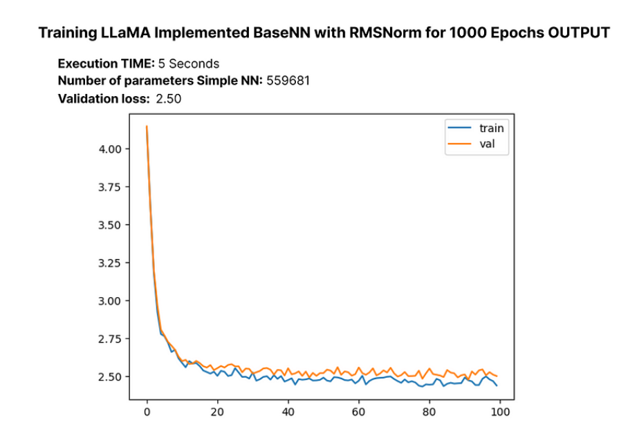
100个epoch后验证损失略有减少，更新后的 LLM 参数总数约为 55 000 个。

14.RoPE效果验证

接下来，我们将实现旋转位置嵌入。在 RoPE 中，作者建议通过旋转嵌入来嵌入序列中Token的位置信息，并在每个位置应用不同的旋转。让我们创建一个函数，模仿论文中 RoPE 的实际实现：

def get_rotary_matrix(context_window, embedding_dim):    # Initialize a tensor for the rotary matrix with zeros    R = torch.zeros((context_window, embedding_dim, embedding_dim), requires_grad=False)
    # Loop through each position in the context window    for position in range(context_window):        # Loop through each dimension in the embedding        for i in range(embedding_dim // 2):            # Calculate the rotation angle (theta) based on the position and embedding dimension            theta = 10000. ** (-2. * (i - 1) / embedding_dim)            # Calculate the rotated matrix elements using sine and cosine functions            m_theta = position * theta            R[position, 2 * i, 2 * i] = np.cos(m_theta)            R[position, 2 * i, 2 * i + 1] = -np.sin(m_theta)            R[position, 2 * i + 1, 2 * i] = np.sin(m_theta)            R[position, 2 * i + 1, 2 * i + 1] = np.cos(m_theta)    return R

我们根据指定的上下文窗口和嵌入维度，按照建议的 RoPE 实现方法生成旋转矩阵。

大家可能对Transformer的架构并不陌生，其中涉及注意力头，因此在实现 LLaMA 时，我们同样需要创建注意力头。此外，为了清晰起见，每一行都有注释：

class RoPEAttentionHead(nn.Module):    def __init__(self, config):        super().__init__()        self.config = config        # Linear transformation for query        self.w_q = nn.Linear(config['d_model'], config['d_model'], bias=False)        # Linear transformation for key        self.w_k = nn.Linear(config['d_model'], config['d_model'], bias=False)        # Linear transformation for value        self.w_v = nn.Linear(config['d_model'], config['d_model'], bias=False)        # Obtain rotary matrix for positional embeddings        self.R = get_rotary_matrix(config['context_window'], config['d_model'])    def get_rotary_matrix(context_window, embedding_dim):        # Generate rotational matrix for RoPE        R = torch.zeros((context_window, embedding_dim, embedding_dim), requires_grad=False)        for position in range(context_window):            for i in range(embedding_dim//2):
                # Rest of the code                ...        return R    def forward(self, x, return_attn_weights=False):        # x: input tensor of shape (batch, sequence length, dimension)        b, m, d = x.shape  # batch size, sequence length, dimension        # Linear transformations for Q, K, and V        q = self.w_q(x)        k = self.w_k(x)        v = self.w_v(x)        # Rotate Q and K using the RoPE matrix        q_rotated = (torch.bmm(q.transpose(0, 1), self.R[:m])).transpose(0, 1)        k_rotated = (torch.bmm(k.transpose(0, 1), self.R[:m])).transpose(0, 1)        # Perform scaled dot-product attention        activations = F.scaled_dot_product_attention(            q_rotated, k_rotated, v, dropout_p=0.1, is_causal=True        )        if return_attn_weights:            # Create a causal attention mask            attn_mask = torch.tril(torch.ones((m, m)), diagonal=0)            # Calculate attention weights and add causal mask            attn_weights = torch.bmm(q_rotated, k_rotated.transpose(1, 2)) / np.sqrt(d) + attn_mask            attn_weights = F.softmax(attn_weights, dim=-1)            return activations, attn_weights        return activations

现在，我们有了一个返回注意力权重的单头屏蔽注意力头，下一步就是创建一个多头注意力机制。

class RoPEMaskedMultiheadAttention(nn.Module):    def __init__(self, config):        super().__init__()        self.config = config        # Create a list of RoPEMaskedAttentionHead instances as attention heads        self.heads = nn.ModuleList([            RoPEMaskedAttentionHead(config) for _ in range(config['n_heads'])        ])        self.linear = nn.Linear(config['n_heads'] * config['d_model'], config['d_model'])  # Linear layer after concatenating heads        self.dropout = nn.Dropout(.1)  # Dropout layer    def forward(self, x):        # x: input tensor of shape (batch, sequence length, dimension)        # Process each attention head and concatenate the results        heads = [h(x) for h in self.heads]        x = torch.cat(heads, dim=-1)
        # Apply linear transformation to the concatenated output        x = self.linear(x)
        # Apply dropout        x = self.dropout(x)        return x

原论文在较小的 7b LLM 变体中使用了 32 个head，但由于条件限制，我们的方法将使用 8 个head。

# Update the master configuration with the number of attention headsMASTER_CONFIG.update({    'n_heads': 8,})

现在我们已经实现了旋转位置嵌入和多头注意力，让我们用更新后的代码重新编写 RMSNorm 神经网络模型。我们将测试其性能、计算损失并检查参数数量。我们将把更新后的模型称为 “RopeModel”。

class RopeModel(nn.Module):    def __init__(self, config):        super().__init__()        self.config = config        # Embedding layer for input tokens        self.embedding = nn.Embedding(config['vocab_size'], config['d_model'])
        # RMSNorm layer for pre-normalization        self.rms = RMSNorm((config['context_window'], config['d_model']))
        # RoPEMaskedMultiheadAttention layer        self.rope_attention = RoPEMaskedMultiheadAttention(config)        # Linear layer followed by ReLU activation        self.linear = nn.Sequential(            nn.Linear(config['d_model'], config['d_model']),            nn.ReLU(),        )        # Final linear layer for prediction        self.last_linear = nn.Linear(config['d_model'], config['vocab_size'])        print("model params:", sum([m.numel() for m in self.parameters()]))    def forward(self, idx, targets=None):        # idx: input indices        x = self.embedding(idx)        # One block of attention        x = self.rms(x)  # RMS pre-normalization        x = x + self.rope_attention(x)        x = self.rms(x)  # RMS pre-normalization        x = x + self.linear(x)        logits = self.last_linear(x)        if targets is not None:            loss = F.cross_entropy(logits.view(-1, self.config['vocab_size']), targets.view(-1))            return logits, loss        else:            return logits

让我们使用 RMSNorm、旋转位置嵌入和多头注意力来执行修改后的 NN 模型，以观察模型中参数数量的更新情况以及损失情况：

# Create an instance of RopeModel (RMSNorm, RoPE, Multi-Head)model = RopeModel(MASTER_CONFIG)# Obtain batches for trainingxs, ys = get_batches(dataset, 'train', MASTER_CONFIG['batch_size'], MASTER_CONFIG['context_window'])# Calculate logits and loss using the modellogits, loss = model(xs, ys)# Define the Adam optimizer for model parametersoptimizer = torch.optim.Adam(model.parameters())# Train the modeltrain(model, optimizer)

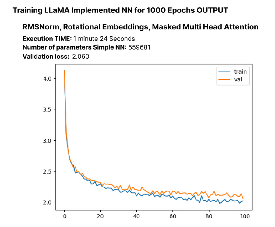
100个epoch后验证损失再次出现小幅下降，更新后的 LLM 参数总数约为 55 000。让我们对模型进行更多的epoch训练，看看重新创建的 LLaMA LLM 的损失是否会继续减少。

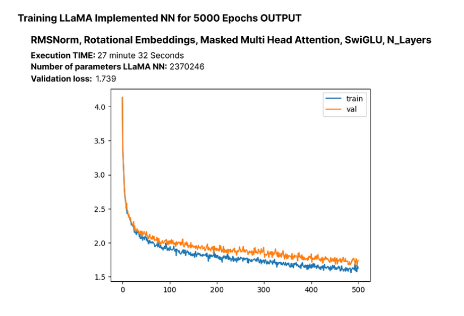
# Updating training configuration with more epochs and a logging intervalMASTER_CONFIG.update({    "epochs": 5000,    "log_interval": 10,})# Training the model with the updated configurationtrain(model, optimizer)

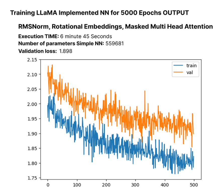
500个epoch后验证损失继续减少，这表明进行更多的epoch训练可以进一步减少损失，尽管减少的幅度不大。

15.采用SwiGLU激活函数

如前所述，LLaMA 的创建者使用 SwiGLU 而不是 ReLU，因此我们将在代码中实现 SwiGLU 方程。

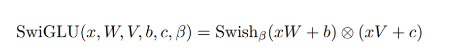
代码实现如下：

class SwiGLU(nn.Module):    """ Paper Link -> https://arxiv.org/pdf/2002.05202v1.pdf """    def __init__(self, size):        super().__init__()        self.config = config  # Configuration information        self.linear_gate = nn.Linear(size, size)  # Linear transformation for the gating mechanism        self.linear = nn.Linear(size, size)  # Linear transformation for the main branch        self.beta = torch.randn(1, requires_grad=True)  # Random initialization of the beta parameter        # Using nn.Parameter for beta to ensure it's recognized as a learnable parameter        self.beta = nn.Parameter(torch.ones(1))        self.register_parameter("beta", self.beta)    def forward(self, x):        # Swish-Gated Linear Unit computation        swish_gate = self.linear_gate(x) * torch.sigmoid(self.beta * self.linear_gate(x))        out = swish_gate * self.linear(x)  # Element-wise multiplication of the gate and main branch        return out

接着我们需要将其集成到修改后的 LLaMA 语言模型（RopeModel）中。

class RopeModel(nn.Module):    def __init__(self, config):        super().__init__()        self.config = config        # Embedding layer for input tokens        self.embedding = nn.Embedding(config['vocab_size'], config['d_model'])
        # RMSNorm layer for pre-normalization        self.rms = RMSNorm((config['context_window'], config['d_model']))
        # Multi-head attention layer with RoPE (Rotary Positional Embeddings)        self.rope_attention = RoPEMaskedMultiheadAttention(config)        # Linear layer followed by SwiGLU activation        self.linear = nn.Sequential(            nn.Linear(config['d_model'], config['d_model']),            SwiGLU(config['d_model']),  # Adding SwiGLU activation        )        # Output linear layer        self.last_linear = nn.Linear(config['d_model'], config['vocab_size'])        # Printing total model parameters        print("model params:", sum([m.numel() for m in self.parameters()]))    def forward(self, idx, targets=None):        x = self.embedding(idx)        # One block of attention        x = self.rms(x)  # RMS pre-normalization        x = x + self.rope_attention(x)        x = self.rms(x)  # RMS pre-normalization        x = x + self.linear(x)  # Applying SwiGLU activation        logits = self.last_linear(x)        if targets is not None:            # Calculate cross-entropy loss if targets are provided            loss = F.cross_entropy(logits.view(-1, self.config['vocab_size']), targets.view(-1))            return logits, loss        else:            return logits

让我们使用 RMSNorm、旋转嵌入、多头注意力和 SwiGLU 来执行修改后的 NN 模型，以观察模型中参数数量的更新情况以及损失情况：

# Create an instance of RopeModel (RMSNorm, RoPE, Multi-Head, SwiGLU)model = RopeModel(MASTER_CONFIG)# Obtain batches for trainingxs, ys = get_batches(dataset, 'train', MASTER_CONFIG['batch_size'], MASTER_CONFIG['context_window'])# Calculate logits and loss using the modellogits, loss = model(xs, ys)# Define the Adam optimizer for model parametersoptimizer = torch.optim.Adam(model.parameters())# Train the modeltrain(model, optimizer)

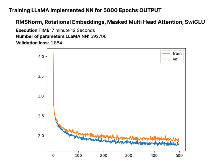
在训练500个epoch后，验证损失再次出现小幅下降，更新后的 LLM 参数总数约为 60,000 个。

到目前为止，我们已经成功实现了本文的关键部分，即 RMSNorm、RoPE 和 SwiGLU。我们注意到，这些实施方法使损失减少到最低程度。

16.扩大模型规模

现在，我们将为 LLaMA 增加层数，以检验其对损失的影响。原论文的 7b 版本使用了 32 个Transformer Block Layer，但我们将只使用 4 个。让我们相应地调整模型设置。

# Update model configurations for the number of layersMASTER_CONFIG.update({    'n_layers': 4,  # Set the number of layers to 4})

让我们先创建一个Transformer Block，了解它的影响。

# add RMSNorm and residual connectionclass LlamaBlock(nn.Module):    def __init__(self, config):        super().__init__()        self.config = config        # RMSNorm layer        self.rms = RMSNorm((config['context_window'], config['d_model']))        # RoPE Masked Multihead Attention layer        self.attention = RoPEMaskedMultiheadAttention(config)        # Feedforward layer with SwiGLU activation        self.feedforward = nn.Sequential(            nn.Linear(config['d_model'], config['d_model']),            SwiGLU(config['d_model']),        )    def forward(self, x):        # one block of attention        x = self.rms(x) # RMS pre-normalization        x = x + self.attention(x)  # residual connection        x = self.rms(x) # RMS pre-normalization        x = x + self.feedforward(x)  # residual connection        return x

创建 LlamaBlock 类的实例，并将其应用于随机张量。

# Create an instance of the LlamaBlock class with the provided configurationblock = LlamaBlock(MASTER_CONFIG)# Generate a random tensor with the specified batch size, context window, and model dimensionrandom_input = torch.randn(MASTER_CONFIG['batch_size'], MASTER_CONFIG['context_window'], MASTER_CONFIG['d_model'])# Apply the LlamaBlock to the random input tensoroutput = block(random_input)

在成功创建了单层之后，我们现在可以用它来构建多层。此外，我们将把模型类从 "ropemodel "更名为 “Llama”，因为我们已经实现了 LLaMA 语言模型的每个组件。

class Llama(nn.Module):    def __init__(self, config):        super().__init__()        self.config = config        # Embedding layer for token representations        self.embeddings = nn.Embedding(config['vocab_size'], config['d_model'])        # Sequential block of LlamaBlocks based on the specified number of layers        self.llama_blocks = nn.Sequential(            OrderedDict([(f"llama_{i}", LlamaBlock(config)) for i in range(config['n_layers'])])        )        # Feedforward network (FFN) for final output        self.ffn = nn.Sequential(            nn.Linear(config['d_model'], config['d_model']),            SwiGLU(config['d_model']),            nn.Linear(config['d_model'], config['vocab_size']),        )        # Print total number of parameters in the model        print("model params:", sum([m.numel() for m in self.parameters()]))    def forward(self, idx, targets=None):        # Input token indices are passed through the embedding layer        x = self.embeddings(idx)        # Process the input through the LlamaBlocks        x = self.llama_blocks(x)        # Pass the processed input through the final FFN for output logits        logits = self.ffn(x)        # If targets are not provided, return only the logits        if targets is None:            return logits        # If targets are provided, compute and return the cross-entropy loss        else:            loss = F.cross_entropy(logits.view(-1, self.config['vocab_size']), targets.view(-1))            return logits, loss

让我们使用 RMSNorm、旋转嵌入、多头注意力、SwiGLU 和 N_layers 执行修改后的 LLaMA 模型，以观察模型中更新的参数数量和损失：

# Create an instance of RopeModel (RMSNorm, RoPE, Multi-Head, SwiGLU, N_layers)llama = Llama(MASTER_CONFIG)# Obtain batches for trainingxs, ys = get_batches(dataset, 'train', MASTER_CONFIG['batch_size'], MASTER_CONFIG['context_window'])# Calculate logits and loss using the modellogits, loss = llama(xs, ys)# Define the Adam optimizer for model parametersoptimizer = torch.optim.Adam(llama.parameters())# Train the modeltrain(llama, optimizer)

虽然存在过拟合的可能性，但关键是要探索延长epoch数目是否会进一步减少损失。此外，请注意我们目前的 LLM 有 200 多万个参数。

让我们用更多的epoch来训练它。

# Update the number of epochs in the configurationMASTER_CONFIG.update({    'epochs': 10000,})# Train the LLaMA model for the specified number of epochstrain(llama, optimizer, scheduler=None, config=MASTER_CONFIG

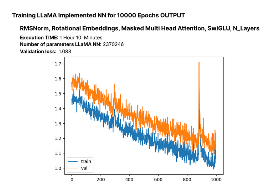
这里的损失为 1.08，我们可以获得更低的损失，而不会遇到明显的过拟合。这表明该模型表现良好。

17.推理验证

到目前为止，我们已经在自定义数据集上成功实现了 LLaMA 架构的缩小版。现在，让我们检查一下 200 万参数语言模型的生成输出。

# Generate text using the trained LLM (llama) with a maximum of 500 tokensgenerated_text = generate(llama, MASTER_CONFIG, 500)[0]print(generated_text)

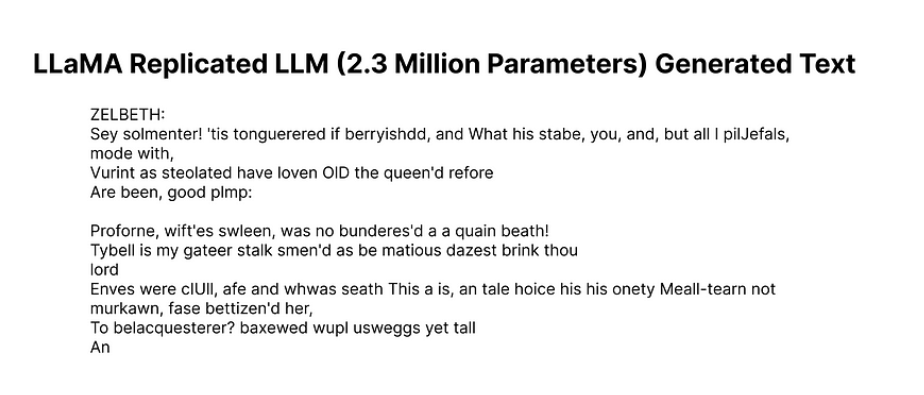
尽管生成的一些单词可能不是完美的英语，但我们的 LLM 仅用 200 万个参数就显示出了对英语的基本理解。

现在，让我们看看我们的模型在测试集上的表现如何。

# Get batches from the test setxs, ys = get_batches(dataset, 'test', MASTER_CONFIG['batch_size'], MASTER_CONFIG['context_window'])# Pass the test data through the LLaMA modellogits, loss = llama(xs, ys)# Print the loss on the test setprint(loss)

测试集的计算损失约为 1.236。

18.超参数实验

超参数调整是训练神经网络的关键步骤。在最初的 Llama 论文中，作者使用了余弦退火学习策略。然而，在我们的实验中，它的表现并不理想。下面是一个使用不同学习策略进行超参数实验的例子：

# Update configurationMASTER_CONFIG.update({    "epochs": 1000})# Create Llama model with Cosine Annealing learning schedulellama_with_cosine = Llama(MASTER_CONFIG)# Define Adam optimizer with specific hyperparametersllama_optimizer = torch.optim.Adam(    llama.parameters(),    betas=(.9, .95),    weight_decay=.1,    eps=1e-9,    lr=1e-3)# Define Cosine Annealing learning rate schedulerscheduler = torch.optim.lr_scheduler.CosineAnnealingLR(llama_optimizer, 300, eta_min=1e-5)# Train the Llama model with the specified optimizer and schedulertrain(llama_with_cosine, llama_optimizer, scheduler=scheduler)

19.保存模型

大家可以使用以下方法保存整个 LLM ：

# Save the entire modeltorch.save(llama, 'llama_model.pth')# If you want to save only the model parameterstorch.save(llama.state_dict(), 'llama_model_params.pth')

要为 Hugging Face 的 Transformers 库保存 PyTorch 模型，可以使用 save_pretrained 方法。下面是一个例子：

from transformers import GPT2LMHeadModel, GPT2Config# Assuming Llama is your PyTorch modelllama_config = GPT2Config.from_dict(MASTER_CONFIG)llama_transformers = GPT2LMHeadModel(config=llama_config)llama_transformers.load_state_dict(llama.state_dict())# Specify the directory where you want to save the modeloutput_dir = "llama_model_transformers"# Save the model and configurationllama_transformers.save_pretrained(output_dir)

GPT2Config 用于创建与 GPT-2 兼容的配置对象。然后，创建 GPT2LMHeadModel 并加载 Llama 模型的权重。最后，调用 save_pretrained 将模型和配置保存在指定目录中。

然后就可以使用Transformer库加载模型了：

from transformers import GPT2LMHeadModel, GPT2Config# Specify the directory where the model was savedoutput_dir = "llama_model_transformers"# Load the model and configurationllama_transformers = GPT2LMHeadModel.from_pretrained(output_dir)

20.结论

在本文中，我们逐步介绍如何采用 LLaMA 方法来构建自己的小型语言模型 (LLM)。作为建议，您可以考虑将模型扩展到 1,500 万个参数左右，因为 1,000 万到 2,000 万个参数范围内的小型模型往往能更好地理解英语。

如何学习大模型 AI ？

由于新岗位的生产效率，要优于被取代岗位的生产效率，所以实际上整个社会的生产效率是提升的。

但是具体到个人，只能说是：

“最先掌握AI的人，将会比较晚掌握AI的人有竞争优势”。

这句话，放在计算机、互联网、移动互联网的开局时期，都是一样的道理。

我在一线互联网企业工作十余年里，指导过不少同行后辈。帮助很多人得到了学习和成长。

我意识到有很多经验和知识值得分享给大家，也可以通过我们的能力和经验解答大家在人工智能学习中的很多困惑，所以在工作繁忙的情况下还是坚持各种整理和分享。但苦于知识传播途径有限，很多互联网行业朋友无法获得正确的资料得到学习提升，故此将并将重要的AI大模型资料包括AI大模型入门学习思维导图、精品AI大模型学习书籍手册、视频教程、实战学习等录播视频免费分享出来。

在这里插入图片描述