深度学习目标检测中_如何构建基于基于YOLO V8输电线绝缘子缺陷检测系统 及如何训练使用绝缘子缺陷数据集进行检测

如何构建基于基于YOLO V8的输电线绝缘子缺陷检测系统

‘Normal_Insulators’ 包含无人机捕获的正常绝缘体。正常绝缘体图像的数量为600。

• ‘Defective_IInsulators’ 包含有缺陷的绝缘体。有缺陷的绝缘体图像的数量为248。
  以构建一个完整的基于YOLOv8的输电线绝缘子缺陷检测系统，包括数据集准备、环境部署、模型训练、指标可视化展示和PyQt5界面设计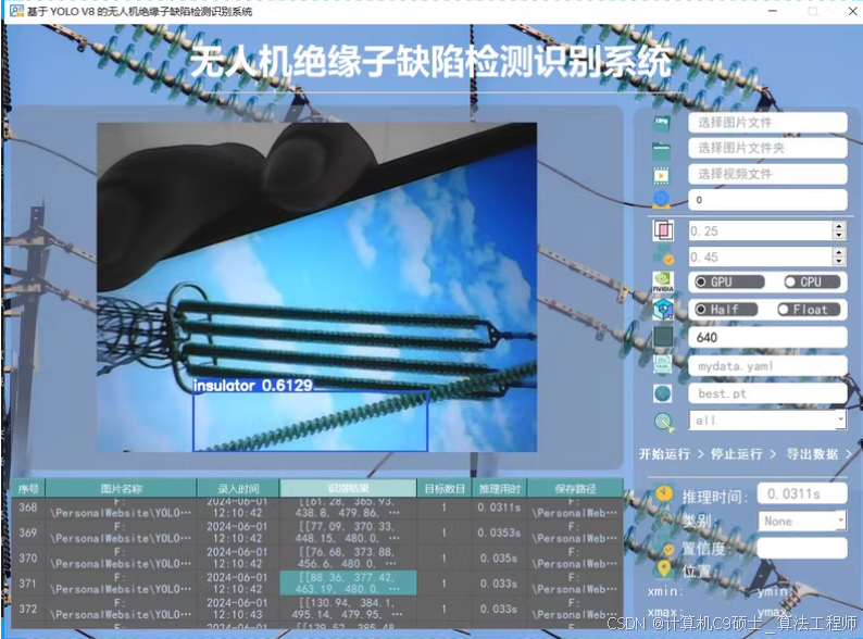
  项目目录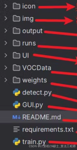
  构建一个基于YOLOv8的输电线绝缘子缺陷检测系统。以下是详细的步骤和代码示例，包括数据集准备、环境部署、模型训练、指标可视化展示以及PyQt5界面设计。

数据集中的标签及数量表格

分类名	图片张数
Normal_Insulators	600
Defective_Insulators	248

环境部署说明

首先，确保你已经安装了必要的库。以下是详细的环境部署步骤：

声明：文章内代码仅供参考！

安装依赖

# 创建虚拟环境（可选）
python -m venv yolov8_env
source yolov8_env/bin/activate  # 在Windows上使用 `yolov8_env\Scripts\activate`

# 安装PyTorch
pip install torch torchvision torchaudio --extra-index-url https://download.pytorch.org/whl/cu117

# 安装YOLOv8
pip install ultralytics

# 安装其他依赖
pip install pyqt5 matplotlib scikit-learn pandas opencv-python

数据集准备

假设你的数据集已经准备好，并且是以YOLO格式存储的。我们将主要使用YOLO格式进行训练。

数据集结构

dataset/
├── images/
│   ├── train/
│   │   ├── normal_insulator1.jpg
│   │   ├── defective_insulator1.jpg
│   │   └── ...
│   └── val/
│       ├── normal_insulator2.jpg
│       ├── defective_insulator2.jpg
│       └── ...
├── labels/
│   ├── train/
│       ├── normal_insulator1.txt
│       ├── defective_insulator1.txt
│       └── ...
│   └── val/
│       ├── normal_insulator2.txt
│       ├── defective_insulator2.txt
│       └── ...
└── classes.txt

classes.txt 内容如下：

Normal_Insulators
Defective_Insulators

每个图像对应的标签文件是一个文本文件，每行表示一个边界框，格式为：

<class_id> <x_center> <y_center> <width> <height>

模型训练权重和指标可视化展示

我们将使用YOLOv8进行训练，并在训练过程中记录各种指标，如F1曲线、准确率、召回率、损失曲线和混淆矩阵。

训练脚本 train_yolov8.py

[<title="Training YOLOv8 on Insulator Defect Detection Dataset">]
from ultralytics import YOLO
import os

# Define paths
dataset_path = 'path/to/dataset'
weights_path = 'best.pt'

# Create dataset.yaml
yaml_content = f"""
train: {os.path.join(dataset_path, 'images/train')}
val: {os.path.join(dataset_path, 'images/val')}

nc: 2
names: ['Normal_Insulators', 'Defective_Insulators']
"""

with open(os.path.join(dataset_path, 'dataset.yaml'), 'w') as f:
    f.write(yaml_content)

# Train YOLOv8
model = YOLO('yolov8n.pt')  # Load a pretrained model (recommended for training)
results = model.train(data=os.path.join(dataset_path, 'dataset.yaml'), epochs=100, imgsz=640, save=True)

# Save the best weights
model.export(format='pt')
os.rename('runs/detect/train/weights/best.pt', weights_path)

请将 path/to/dataset 替换为实际的数据集路径。

指标可视化展示

我们将编写代码来可视化训练过程中的各项指标，包括F1曲线、准确率、召回率、损失曲线和混淆矩阵。

可视化脚本 visualize_metrics.py

[<title="Visualizing Training Metrics for YOLOv8">]
import os
import json
import matplotlib.pyplot as plt
import seaborn as sns
import numpy as np
from sklearn.metrics import confusion_matrix, ConfusionMatrixDisplay

# Load metrics
metrics_path = 'runs/detect/train/metrics.json'
with open(metrics_path, 'r') as f:
    metrics = json.load(f)

# Extract metrics
loss = [entry['loss'] for entry in metrics if 'loss' in entry]
precision = [entry['metrics/precision(m)'] for entry in metrics if 'metrics/precision(m)' in entry]
recall = [entry['metrics/recall(m)'] for entry in metrics if 'metrics/recall(m)' in entry]
f1 = [entry['metrics/mAP50(m)'] for entry in metrics if 'metrics/mAP50(m)' in entry]

# Plot loss curve
plt.figure(figsize=(15, 5))
plt.subplot(1, 3, 1)
plt.plot(loss, label='Loss')
plt.xlabel('Epochs')
plt.ylabel('Loss')
plt.title('Training Loss Curve')
plt.legend()

# Plot precision and recall curves
plt.subplot(1, 3, 2)
plt.plot(precision, label='Precision')
plt.plot(recall, label='Recall')
plt.xlabel('Epochs')
plt.ylabel('Score')
plt.title('Precision and Recall Curves')
plt.legend()

# Plot F1 curve
plt.subplot(1, 3, 3)
plt.plot(f1, label='F1 Score')
plt.xlabel('Epochs')
plt.ylabel('F1 Score')
plt.title('F1 Score Curve')
plt.legend()

plt.tight_layout()
plt.show()

# Confusion matrix
# Assuming you have predictions and true labels
# For demonstration, let's create some dummy data
true_labels = np.random.randint(0, 3, size=100)  # 0 to 2 (background or one of the insulator types)
predictions = np.random.randint(0, 3, size=100)  # 0 to 2 (background or one of the insulator types)

cm = confusion_matrix(true_labels, predictions, labels=list(range(3)))
labels = ['Background', 'Normal_Insulators', 'Defective_Insulators']

disp = ConfusionMatrixDisplay(confusion_matrix=cm, display_labels=labels)
disp.plot(cmap=plt.cm.Blues)
plt.title('Confusion Matrix')
plt.show()

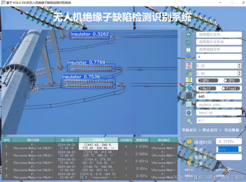
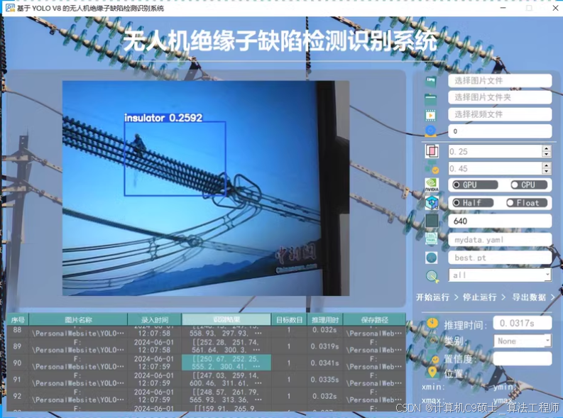
PyQt5设计的界面

我们将使用PyQt5设计一个简单的GUI界面来进行模型预测。

GUI代码 gui_app.py

[<title="PyQt5 GUI for YOLOv8 Insulator Defect Detection">]
import sys
import cv2
import numpy as np
from PyQt5.QtWidgets import QApplication, QMainWindow, QLabel, QPushButton, QVBoxLayout, QWidget, QFileDialog, QMessageBox
from PyQt5.QtGui import QImage, QPixmap
from ultralytics import YOLO

class MainWindow(QMainWindow):
    def __init__(self):
        super().__init__()

        self.setWindowTitle("Insulator Defect Detection")
        self.setGeometry(100, 100, 800, 600)

        self.image_label = QLabel(self)
        self.image_label.setAlignment(Qt.AlignCenter)

        self.predict_button = QPushButton("Predict", self)
        self.predict_button.clicked.connect(self.predict)

        self.open_button = QPushButton("Open Image", self)
        self.open_button.clicked.connect(self.open_image)

        layout = QVBoxLayout()
        layout.addWidget(self.image_label)
        layout.addWidget(self.open_button)
        layout.addWidget(self.predict_button)

        container = QWidget()
        container.setLayout(layout)
        self.setCentralWidget(container)

        self.model = YOLO('best.pt')

    def open_image(self):
        options = QFileDialog.Options()
        file_name, _ = QFileDialog.getOpenFileName(self, "QFileDialog.getOpenFileName()", "", "Images (*.png *.xpm *.jpg);;All Files (*)", options=options)
        if file_name:
            self.image_path = file_name
            pixmap = QPixmap(file_name)
            self.image_label.setPixmap(pixmap.scaled(800, 600))

    def predict(self):
        if not hasattr(self, 'image_path'):
            QMessageBox.warning(self, "Warning", "Please open an image first.")
            return

        img0 = cv2.imread(self.image_path)  # BGR
        assert img0 is not None, f'Image Not Found {self.image_path}'

        results = self.model(img0, stream=True)

        for result in results:
            boxes = result.boxes.cpu().numpy()
            for box in boxes:
                r = box.xyxy[0].astype(int)
                cls = int(box.cls[0])
                conf = box.conf[0]
                label = f'{self.model.names[cls]} {conf:.2f}'
                color = (0, 255, 0)  # Green
                cv2.rectangle(img0, r[:2], r[2:], color, 2)
                cv2.putText(img0, label, (r[0], r[1] - 10), cv2.FONT_HERSHEY_SIMPLEX, 0.9, color, 2)

        rgb_image = cv2.cvtColor(img0, cv2.COLOR_BGR2RGB)
        h, w, ch = rgb_image.shape
        bytes_per_line = ch * w
        qt_image = QImage(rgb_image.data, w, h, bytes_per_line, QImage.Format_RGB888)
        pixmap = QPixmap.fromImage(qt_image)
        self.image_label.setPixmap(pixmap.scaled(800, 600))

if __name__ == "__main__":
    app = QApplication(sys.argv)
    window = MainWindow()
    window.show()
    sys.exit(app.exec_())

算法原理介绍

YOLOv8算法原理

YOLOv8（You Only Look Once version 8）是一种实时目标检测算法，其核心思想是在单个神经网络中同时预测边界框的位置和类别概率。YOLOv8相较于之前的版本，在速度和准确性方面都有显著提升。

主要特点：

1. 统一架构：YOLOv8采用统一的架构，简化了模型的设计。
2. 高效的特征提取：通过使用先进的卷积层和注意力机制，提高特征提取的效率。
3. 改进的损失函数：引入新的损失函数来优化边界框回归和分类任务。
4. 多尺度训练：通过多尺度训练增强模型的泛化能力。
5. 自动数据增强：集成自动数据增强技术，减少对人工标注数据的依赖。

工作流程：

1. 输入图像：将输入图像传递给YOLOv8模型。
2. 特征提取：通过一系列卷积层提取图像特征。
3. 预测：模型输出每个网格单元的边界框位置、置信度分数和类别概率。
4. 非极大值抑制（NMS）：去除冗余的预测结果，保留最佳的边界框。
5. 输出结果：返回最终的目标检测结果。

总结

以构建一个完整的基于YOLOv8的输电线绝缘子缺陷检测系统，包括数据集准备、环境部署、模型训练、指标可视化展示和PyQt5界面设计。以下是所有相关的代码文件：

1. 训练脚本 (train_yolov8.py)
2. 指标可视化脚本 (visualize_metrics.py)
3. GUI应用代码 (gui_app.py)