【 MATLAB 】legend 的使用简析

目录

legend

在作图命令中（plot）给出图例标签；

legend(label1,...,labelN)

给当前轴添加图例；

legend(target,___)

给特定轴添加图例；

legend(subset,___)

给部分函数添加图例；

legend(___,'Location',lcn)

指定图例的位置（方向）以及显示的列数；

lgd = legend(___)

给图例添加标题；

legend('boxoff')

去除图例边框；

Modify Legend Appearance

修改图例的外观；

---

MATLAB 中 legend 可以翻译为图例，下面逐一用例子来说明 legend 的用法，并辅以必要的说明。

我只挑选几种使用的来说明。

---

legend

在作图命令中（plot）给出图例标签；

Plot two lines. Specify the legend labels during the plotting commands by setting the DisplayName property to the desired text. Then, add a legend.

画两条线。 通过将DisplayName属性设置为所需文本，在绘图命令期间指定图例标签。 然后，添加一个图例（legend）。

% Plot two lines. 
% Specify the legend labels during the plotting commands by setting the DisplayName property to the desired text. 
% Then, add a legend.

clear
clc
close all

x = linspace(0,pi);
y1 = cos(x);
plot(x,y1,'DisplayName','cos(x)')

hold on 
y2 = cos(2*x);
plot(x,y2,'DisplayName','cos(2x)')
hold off

legend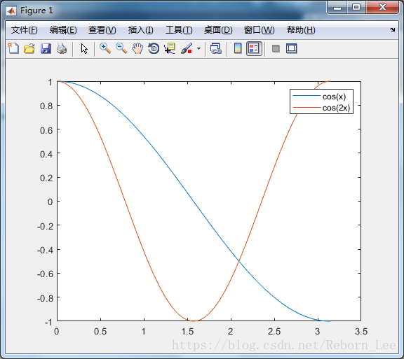

对代码做如下改动，将两幅图分开画，然后添加图例的方法：

% Plot two lines. 
% Specify the legend labels during the plotting commands by setting the DisplayName property to the desired text. 
% Then, add a legend.

clear
clc
close all

x = linspace(0,pi);
y1 = cos(x);
subplot(2,1,1);
plot(x,y1,'DisplayName','cos(x)')

legend

%hold on 
y2 = cos(2*x);
subplot(2,1,2);
plot(x,y2,'DisplayName','cos(2x)')
% hold off

legend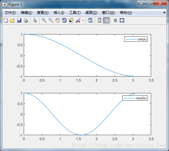

---

legend(label1,...,labelN)

给当前轴添加图例；

legend(label1,...,labelN) sets the legend labels. Specify the labels as a list of character vectors or strings, such as legend('Jan','Feb','Mar').

legend（label1，...，labelN）设置图例标签。 将标签指定为字符向量或字符串列表，例如legend（'Jan'，'Feb'&#x