[论文精读]Learning Dynamic Graph Representation of Brain Connectome with Spatio-Temporal Attention

夏莉莉iy

已于 2024-03-21 13:01:37 修改

阅读量404

点赞数 2

分类专栏：论文精读文章标签：深度学习人工智能计算机视觉学习机器学习 transformer 笔记

于 2023-10-03 22:56:26 首次发布

本文链接：https://blog.csdn.net/Sherlily/article/details/133527837

版权

论文精读专栏收录该内容

52 篇文章 7 订阅

订阅专栏

论文原文：[2105.13495] Learning Dynamic Graph Representation of Brain Connectome with Spatio-Temporal Attention (arxiv.org)

应该是21 Oct 2021那一版（有些pdf下出来是27 May 2021的，两者有些出入）：学习具有时空注意力的大脑连接组的动态图表示 – arXiv虚荣心 (arxiv-vanity.com)

OpenReview：基于时空注意力的脑连接组学习动态图表示 |OpenReview的

作者提供代码：GitHub - egyptdj/stagin: STAGIN: Spatio-Temporal Attention Graph Isomorphism Network

英文是纯手打的！论文原文的summarizing and paraphrasing。可能会出现难以避免的拼写错误和语法错误，若有发现欢迎评论指正！文章偏向于笔记，谨慎食用！

2.3.1. Graph neural network on dynamic graphs

2.3.2. Attention in graph neural networks

2.4. Theory

2.4.1. Problem definition

2.4.2. Graph Isomorphism Network

2.4.3. Encoder-decoder understanding of GNNs

2.5. STAGIN: Spatio-Temporal Attention Graph Isomorphism Network

2.5.1. Dynamic graph definitio

2.5.2. Spatial attention with attention-based READOUT

2.5.3. Temporal attention with Transformer encoder

2.6. Experiment

2.6.1. Dataset

2.6.2. Experimental settings

2.6.3. HCP-Rest: Gender classification

2.6.4. HCP-Task: Task decoding

2.7. Conclusion

3. 知识补充

3.1. Kronecker product

4. Reference List

1. 省流版

1.1. 心得

（1）只能说最开始看到排版就挺绷不住的，表和图都放附录。会议要求吗是

（2）好难啊数学部分，而且引用了很多别人的，在他们论文里面就没有细说

1.2. 论文框架图

2. 原文逐段阅读

2.1. Abstract

①Previous work did not analyse the temporal information of brain images

②Albeit dynamic functional connectivity (FC) was used in research, their works are lack of temporal interpretation and are low in accuracy

③The authors put forward Spatio-Temporal Attention Graph Isomorphism Network (STAGIN) model which based on dynamic image and includes READOUT and Transformer. READOUT function brings spatial interpretation and Transformer brings temporal interpretion for STAGIN.

④Dataset: Human Connectome Project (HCP)-Rest and HCP-Task

2.2. Introduction

①Briefly introduce functional magnetic resonance imaging (fMRI)

②Present current trend, putting GNN in brain image analysis. Most of them adopt model to resting state and tasking state fMRI to classify phenotype or disease

③Deficiencies of other models

④Generally talking'bout their STADIN

⑤我完全没有读懂什么滥用解码？？

Our work holds potential societal impact in that brain decoding methods can be linked to finding neural biomarkers of important phenotypes or diseases. However, potential negative impact related to privacy concerns that arise from abuse or misuse of accurate decoding methods should also be noted. Although our method is yet behind the decoding capability that can be abused or misused, our research cannot still be free from these ethical considerations.

isomorphism n.同构；类质同象；类质同晶型（现象）；同（晶）型性

2.3. Related works

2.3.1. Graph neural network on dynamic graphs

①Dynamic networks might bring changes of nodes and edges, which causes a big challenge

②Unique node encoding and edge feature are what authors want

2.3.2. Attention in graph neural networks

①Attention mechanism presents great in edge computing and scaling node features. Moreover, pooling mechanism is also an application of attention mechanism in brain maps

②Randomly initializing parameters or local graph structures for attention scoring, the authors challenge their effectiveness

vertice n.顶点

2.4. Theory

2.4.1. Problem definition

①Define $G\left ( t \right )=\left ( V\left ( t \right ),E\left ( t \right ) \right )$ is at time $t$ , where $V(t)=\{x_1(t),\ldots,x_N(t)\}$ is $N$ nodes set and $E(t)=\left\{\{x_i(t),x_j(t)\}\mid j\in\mathcal{N}(i),i\in\{1,\ldots N\}\right\}$ is edges set. $\mathcal{N}(i)$ represents the neighborhood of the vertex $x_{i}$

②They define a mapping function:

$f:G_{dyn}\rightarrow(h_{G(1)},\ldots,h_{G(T)})\rightarrow h_{G_{dyn}}\Leftrightarrow g\circ q$

where $G_{\mathrm{dyn}}=(G(1),\ldots,G(T))$ stores $T$ timepoints graphs, $h_{G_{\mathrm{dyn}}}$ is a vector with $D$ dimensions;

$g\quad:G_{\mathrm{dyn}}\to(h_{G(1)},\ldots,h_{G(T)})$ , which represents GNN;

$q\quad:(h_{G(1)},\ldots,h_{G(T)})\to h_{G_{\mathrm{dyn}}}$ , which represents Transformer encoder.

③The authors reckon this function explain the important areas of brain

disentangle vt.使解脱;使摆脱;分清，清理出(混乱的论据、想法等);理顺;解开…的结;使脱出

2.4.2. Graph Isomorphism Network

①A Graph Isomorphism Network (GIN), which is the variant of the GNN, includes AGGREGATE and COMBINE. The authors set AGGREGATE function to extract features from neighbors and COMBINE function to obtain features from the next layer:

$a_v^{(k)}\quad=\textbf{AGGREGATE}^{(k)}\left(\left\{h_u^{(k-1)}:u\in\mathcal{N}(v)\right\}\right)$

$h_v^{(k)}\quad=\textbf{COMBINE}^{(k)}\left(h_v^{(k-1)},a_v^{(k)}\right)\\\\ \: \: =MLP^{(k)}\Big((1+\epsilon^{(k)})\cdot{h}_v^{(k-1)}+\sum_{u\in\mathcal{N}(v)}{h}_u^{(k-1)}\Big)$

where $h_v^{(k)}$ denotes feature vector of node $x$ at layer $k$ and $\epsilon$ is a learnable parameter initialized with 0.

②Reformulated $h_v^{(k)}$ to matrix $H^{(k)}$ :

$H^{(k)}\quad=\sigma\left((\epsilon^{(k)}\cdot I+A)H^{(k-1)}W^{(k)}\right)=\left[{h}_{1}^{(k)},\cdots,{h}_{N}^{(k)}\right]\in\mathbb{R}^{D\times N}$

where $I$ is identity matrix, $A$ is the adjacency matrix between the node features, $W$ is the weights of the MLP layer, $\sigma$ is the nonlinearity function.

③The READOUT function calculates all features in the whole graph

$h_G^{(k)}=\text{READOUT}\Big(\{h_v^{(k)}\mid v\in G\}\Big)=H^{(k)}\phi_{\mathrm{mean}}$

where $\phi_{\mathrm{mean}}$ denotes calculating the mean value of matrix and reforming the matrix to a vector (mean of rows). Or sometimes $\phi_{\mathrm{sum}}^\top=[1,\ldots,1]$ can also be used as a pooling vector. $\phi$ can be regarded as decoder.

2.4.3. Encoder-decoder understanding of GNNs

①The whole method (a) and READOUT module (b):

②Input encoder in $k$ -th layer:

$E^{(k)}=W^{(k)}\otimes(\epsilon^{(k)}\cdot I+A^T)$

where $\bigotimes$ denotes Kronecker product

③Then node feature:

$H^{(k)}=\Sigma^{(k)}E^{(k)\top}\cdots\Sigma^{(1)}E^{(1)\top}\left[x_1,\cdots,x_N\right]$

（为什么又来一个H啊我不是很明白了）

where $\Sigma^{(k)}$ is diagonal matrix with its elements are 0 or 1. This value depends on specific activation pattern.

④The authors prove $\phi_{\mathrm{mean}}$ is decoder:

Firstly we know, $\begin{aligned}h_G^{(k)}&=\quad\mathrm{Vec}\left(h_G^{(k)}\right)=\mathrm{Vec}\left(H^{(k)}\phi_\mathrm{mean}\right)=\left(\phi_\mathrm{mean}^T\otimes I\right)\mathrm{Vec}\left(H^{(k)}\right)\\\\&=\quad\left(\phi_\mathrm{mean}^T\otimes I\right)\Sigma^{(k)}E^{(k)\top}\cdots\Sigma^{(1)}E^{(1)\top}x\end{aligned}$

Then assuming $b_{i}$ is the $i$ -th column of the encoder matrix $E^{(1)}\Sigma^{(1)}\cdots E^{(k)}\Sigma^{(k)}$ , $\tilde{b}_i$ is is the $i$ -th column of the decoder matrix $\left(\phi_{\mathrm{mean}}^T\otimes I\right)$ ;

Change the expression of $h_G^{(k)}$ : $h_G^{(k)}=\sum_i\langle b_i,x\rangle\tilde{b}_i$ ;

Obviously, the $\tilde{b}_i$ is a constant, hence this encoder-decoder is reasonable.

（？？？可能是我注意力机制的数学没学精，常数就代表可以？）

2.5. STAGIN: Spatio-Temporal Attention Graph Isomorphism Network

①(a) presents how to extract features, (b) is a example of dynamic graph structure

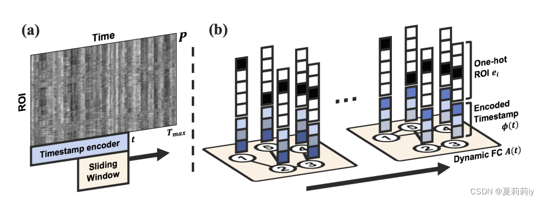
2.5.1. Dynamic graph definitio

①They use 4D fMRI data with 3D voxels across time

②ROI-timeseries matrix $P\in\mathbb{R}^{N\times T_{\max}}$ : mean values of $N$ ROIs at each timepoint

③Stride of sliding-window with length $\Gamma$ is $S$ . $T=\lfloor T_{\max}-\Gamma/S\rfloor$ windowed matrices can be gotten.

④Correlation coefficient matrix of FC at time $t$ :

$R_{ij}(t)=\frac{\mathrm{Cov}(\bar{\boldsymbol{p}}_i(t),\bar{\boldsymbol{p}}_j(t))}{\sigma_{\bar{\boldsymbol{p}}_i}(t)\sigma_{\bar{\boldsymbol{p}}_j}(t)}\in\mathbb{R}^{N\times N}$

where $\bar{p}_i(t)$ and $\bar{p}_j(t)$ are from (a), $\bar{P}(t)\in\mathbb{R}^{N\times\Gamma}$ , $i$ and $j$ are row and column indices respectively, $\mathrm{Cov}$ is cross covariance, $\sigma _{p}$ represents standard deviation of $p$ .

⑤Lastly change $R_{ij}(t)$ to $A(t)\in\{0,1\}^{N\times N}$ by only retaining the top 30% values

⑥To achieve temporal variation, they concatenate encoded timestamp $\eta(t)\in\mathbb{R}^D$ , which is a Gated Recurrent Unit (GRU), to spatial one-hot encoding $e_{v}$

⑦Node features are with learnable parameter matrix $W\in \mathbb{R}^{D\times \left ( N+D \right )}$ :

$x_v(t)=W[e_v||\eta(t)]$

2.5.2. Spatial attention with attention-based READOUT

①The spatial attention:

$z_{space}=s\left ( H \right )$

$\tilde{h}_{G}=Hz_{space}$

where $s:\mathbb{R}^{D\times N}\to[0,1]^N$ is the attention function, $\tilde{h}_{G}$ is spatially attended graph of $h_{G}$ .

②They adopt two attention functions, Graph-Attention READOUT (GARO) and Squeeze-Excitation READOUT (SERO)

（1）GARO: Graph-Attention READOUT

Based on key-query embedding of Transformer, its computing method shows below:

$\begin{aligned} &K=W_\mathrm{key}H \\ &\boldsymbol{q}=\boldsymbol{W_\mathrm{query}}H\boldsymbol{\phi _\mathrm{mean}} \\ \boldsymbol{z_{\mathrm{space}}}&=\operatorname{sigmoid}\bigl(\frac{\boldsymbol{q}^\top\boldsymbol{K}}{\sqrt{D}}\bigr) \end{aligned}$

where $W_{\mathrm{key}}\in\mathbb{R}^{D\times D}$ is learnable key parameter matrix, $W_{\mathrm{query}}\in\mathbb{R}^{D\times D}$ is is learnable query parameter matrix, $K\in\mathbb{R}^{D\times N}$ is the embedded key matrix, $q\in\mathbb{R}^D$ is the embedded query vector.

（2）SERO: Squeeze-Excitation READOUT

The SERO will not scale the channel dimension, but scale the node dimension:

$z_\text{space}\quad=\text{sigmoid}\Big(W_2\sigma(W_1H\phi_\text{mear})\Big)$

where $W_1\in\mathbb{R}^{D\times D},W_2\in\mathbb{R}^{N\times D}$ are learnable parameter matrices.

（3）Orthogonal regularization

For increasing presenting range in $h_{G}$ and decreasing possibility of null subspace within $H$ , they use orthogonal regularization:

$\mathcal{L}_{\mathrm{ortho}}=\left\|1/m\cdot H^\top H-I\right\|_2$

where $m=\max(H^\top H)$ .

2.5.3. Temporal attention with Transformer encoder

Single-headed Transformer encoder for acrossing time:

$h_{G_{\mathrm{dyn}}}=\text{concatenate}(\{h_{G_{\mathrm{dyn}}}^{(k)}|\left.k\in\{1,\ldots,K\}\right\})$

2.6. Experiment

2.6.1. Dataset

①Dataset: HCP S1200 releaseHCP S1200 版本现已在亚马逊云科技上推出 - Connectome (humanconnectome.org)

②Dividing of dataset: HCP-Rest and the HCP-Task

③Pre-process and ICA denoised for HCP-Rest dataset and pre-process for HCP-Task dataset

④Sample: 1093 (female: 594, male: 499) excluding $T_{max}< 1200$ for HCP-Rest and 7450 excluding short time for HCP-Task

⑤Number of classes: $C=2$ for Rest and $7$ for Task

⑥Task: working memory, social, relational, motor, language, gambling, and emotion types

2.6.2. Experimental settings

①Table of two datasets:

②Loss function:

$\mathcal{L}=\mathcal{L}_\mathrm{cross \, \, entropy}+\lambda\cdot\mathcal{L}_\mathrm{ortho}$

where $\lambda$ is scaling coefficient of the orthogonal regularization

③Layers: $K=4$

④Embedding dimension $D=128$

⑤Window length $\Gamma =50$

⑥Window stride $S=3$

⑦regularization coefficient $\lambda=1.0\times10^{-5}$

⑧Capturing FC: 36 seconds every 2.16 seconds (standard)

⑨Dropout rate: 0.5 for $h_{\mathrm{dyn}}$ and 0.1 for $z_{space}$ and $z_{time}$

⑩Activation function: GELU

⑪One-cycle learning rate policy: "learning rate is gradually increased from 0.0005 to 0.001 during the early 20% of the training, and gradually decreased to 5.0×10−7 afterwise"

⑫Epochs: 30 for Rest and 10 for Task

⑬Batch: 3 for Rest and 16 for Task

⑭Cross-validation: 5 fold

⑮Atlas: Schaefer atlas with 400 regions and 7 intrinsic connectivity networks (ICNs)

⑯Dimension of ROI-timeseries: randomly sliced with a fixed length (600 for HCP-Rest, 150 for HCP-Task) for reducing computing time, randomly augmenting data, reducing unwanted memorization, ensuring $T$ across different task labels

⑰Unsliced full matrix $P$ : inference at test time

2.6.3. HCP-Rest: Gender classification

①Goal: classify gender

②Comparison is in 2.6.2. ①

③"Female subjects show hyperconnectivity of the DMN and hypoconnectivity of the SMN when compared to male subjects"

④Temporal attention of the gender classification with k-means clustering:

2.6.4. HCP-Task: Task decoding

①They designed a GLM to analyze the spatially attended regions $z_{space}$ :

$[\boldsymbol{z_\mathrm{space}}(0),\cdots,\boldsymbol{z_\mathrm{space}}(T)]^\top=\boldsymbol{M}[\boldsymbol{\beta_\mathrm{task}},\boldsymbol{\beta_\mathrm{rest}}]^\top+\boldsymbol{\epsilon}$

where $\epsilon$ is residual error

②Mean temporal attention $z_{mean}$ showed in (a) and proportion of statistically significant regions within the 7 ICNs for each layers showed in (b)

2.7. Conclusion

STAGIN peforms great in gender classification through 4D-fMRI

3. 知识补充

3.1. Kronecker product

（1）Definition: two matrices with any shape are able to calculating Kronecker product

（2）Example:

given $A=\begin{bmatrix} a_{11} & a_{12}\\ a_{21} & a_{22} \end{bmatrix}$ , $B= \begin{bmatrix} b_{11} &b_{12} \\ b_{21} & b_{22}\\ b_{31} & b_{32} \end{bmatrix}$

$\begin{aligned} \mathbf{A}\otimes\mathbf{B}= \left.\left[\begin{matrix}{a_{11}\text{ B }a_{12}\text{ B}} \\ { a _ { 21 }\text{B }a_{22}\text{ B}} \end{matrix}\right. \right ] \\ =\begin{bmatrix}a_{11}b_{11}a_{11}b_{12}\, \, \, \, a_{12}b_{11}a_{12}b_{12}\\a_{11}b_{21}a_{11}b_{22}\, \, \, \, a_{12}b_{21}a_{12}b_{22}\\a_{11}b_{31}a_{11}b_{32}\, \, \, \, a_{12}b_{31}a_{12}b_{32}\\ \\a_{21}b_{11}a_{21}b_{12}\, \, \, \, a_{22}b_{11}a_{22}b_{12}\\a_{21}b_{21}a_{21}b_{22}\, \, \, \, a_{22}b_{21}a_{22}\, b_{22}\\a_{21}b_{31}a_{21}b_{32}\, \, \, \, a_{22}b_{31}a_{22}b_{32}\end{bmatrix} \end{aligned}$

（3）Further understanding: 【基础数学】克罗内克内积 Kronecker product-CSDN博客

4. Reference List

Kim, B., Ye, J. & Kim, J. (2021) 'Learning Dynamic Graph Representation of Brain Connectome with Spatio-Temporal Attention', NeurIPS 2021. doi: https://doi.org/10.48550/arXiv.2105.13495

夏莉莉iy

关注

2
点赞
踩
1

收藏

觉得还不错? 一键收藏
2
评论
[论文精读]Learning Dynamic Graph Representation of Brain Connectome with Spatio-Temporal Attention

计算机-人工智能-脑科学与类脑智能
复制链接

扫一扫