[R可视化]数据探索可视化：棘状图和箱线图（以信用卡违约率数据为例）

以信用卡违约率数据为例：

一、客户年龄和信用卡违约的关系

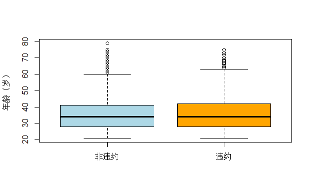
1、不同违约状态下的年龄箱线图

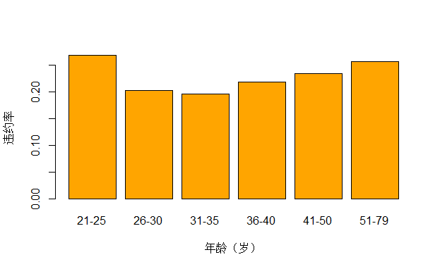
2、不同年龄组（因为年龄的取值过多）的违约率

3、rcode：

#违约率对年龄的分组箱线图
boxplot(X5~Y,data=dta0,col=c("lightblue","orange"),names=c("非违约","违约"),ylab="年龄（岁）")	
#不同年龄的违约率
table(dta0$X5)
#由于年龄取值过多，对年龄分组，计入新的变量age
dta0$age[dta0$X5<=25]<-"21-25"
dta0$age[dta0$X5>25&dta0$X5<=30]<-"26-30"
dta0$age[dta0$X5>30&dta0$X5<=35]<-"31-35"
dta0$age[dta0$X5>35&dta0$X5<=40]<-"36-40"
dta0$age[dta0$X5>40&dta0$X5<=50]<-"41-50"
dta0$age[dta0$X5>50]<-"51-79"
table(dta0$age)
#不同年龄组的违约率图
dta0$default[dta0$Y=="not default"]<-0
dta0$default[dta0$Y=="default"]<-1
table(dta0$default)   ##由于计算违约率时，因变量应该是0-1变量，从而我们构造default变量
barplot(by(dta0$default,dta0$age,mean), col="orange",xlab="年龄（岁）", ylab="违约率")

二、客户个人信息和信用卡违约的关系

1、rcode

#信用卡用户个人信息和违约率关系
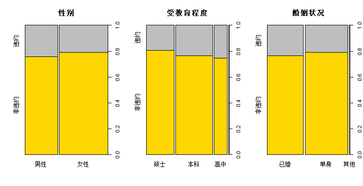
## 画1*3图，分别是性别 vs. 违约，受教育程度 vs. 违约，婚姻状况 VS.违约
par(mfrow=c(1,3))
countGender <- table(dta0$X2, dta0$default)
spineplot(countGender, main="性别", col=c("gold","grey"),xaxlabels=c("男性","女性"),yaxlabels=c("非违约","违约"))
countEducation <- table(dta0$X3, dta0$default)
spineplot(countEducation, main="受教育程度", col=c("gold","grey"),xaxlabels=c("硕士","本科","高中","其他"),yaxlabels=c("非违约","违约"))
countMarriage <- table(dta0$X4, dta0$default)
spineplot(countMarriage, main="婚姻状况", col=c("gold","grey"),xaxlabels=c("已婚","单身","其他"),yaxlabels=c("非违约","违约"))

2、图表：