【Python】Section 6: 多元逻辑回归和缺失值 Multi-logstic Regression and Missingness from HarvardX

1. Multinomial Logistic Regression

There are several extensions to standard logistic regression when the response variable, , has more than two categories. The two most common are:

Ordinal logistic regression: used when the categories have a specific hierarchy (like class year: Freshman, Sophomore, Junior, Senior; or a 7-point rating scale, from Strongly Disagree to Strongly Agree).

Nominal logistic regression: used when the categories have no inherent order (like eye color: blue, green, brown, hazel, etc).

For example, we could attempt to predict a student's concentration

from predictors , number of psets per week, and , time spent in the library.

1.1 One vs. Rest (OVR) Logistic Regression

An option for nominal (non-ordinal) categorical logistic regression model is called the 'One vs. Rest' approach.

If there are 3 classes, then 3 separate logistic regression models are fit. Each model is associated with a specific class and predicts the probability of a given observation belonging to that class as opposed to all the others.

So, for the concentration example, we would fit 3 models:

• a first model to predict CS from Stat and Physics combined,
• a second model to predict Stat from CS and Physics combined,
• a third model to predict Physics from CS and Stat combined.

1.2 A Visual Example of OVR Logistic Regression

Let's say we want to classify observations as belonging to one of three classes: Red, Blue, or Green.

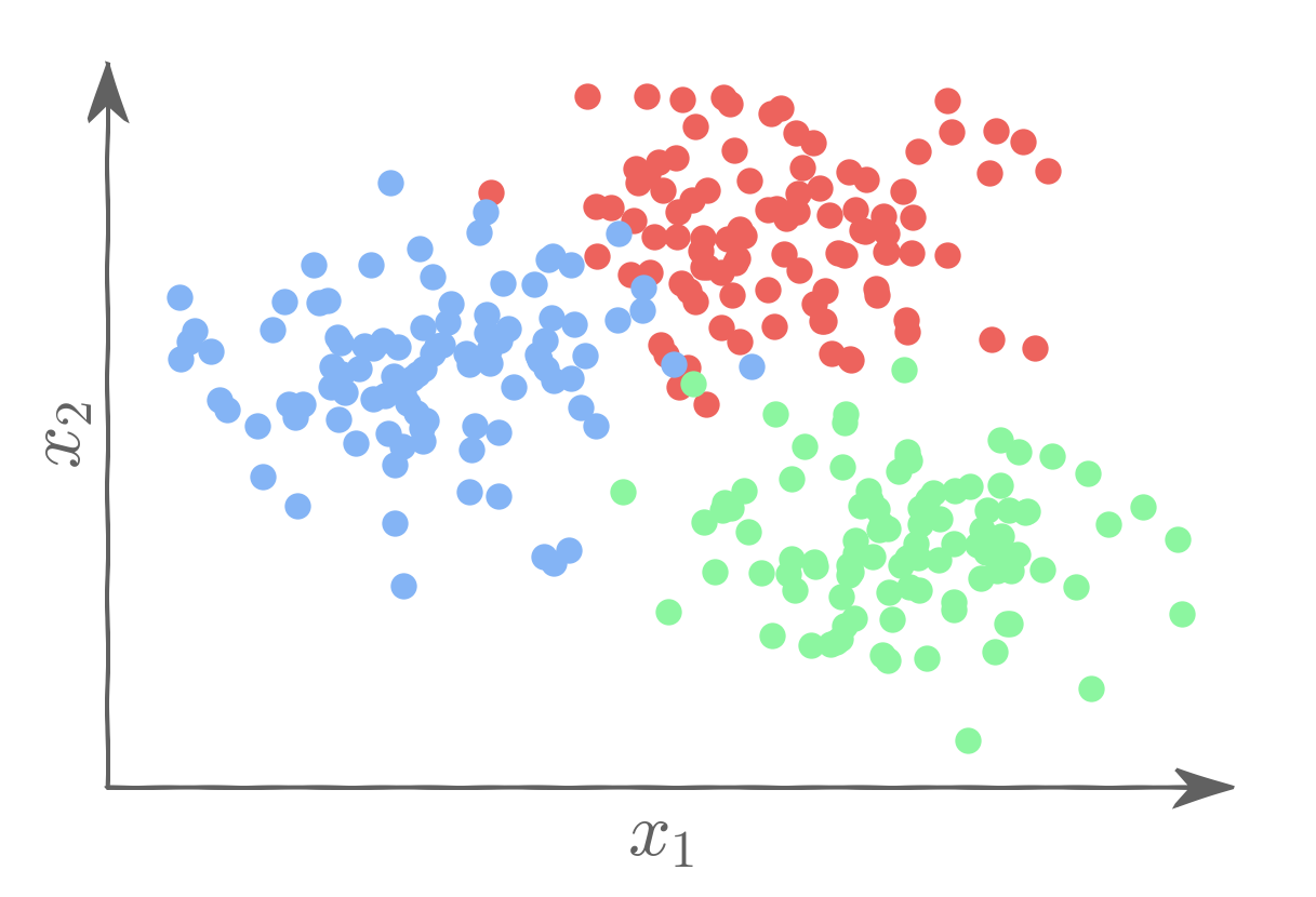
We can then use three binary logistic regression models:

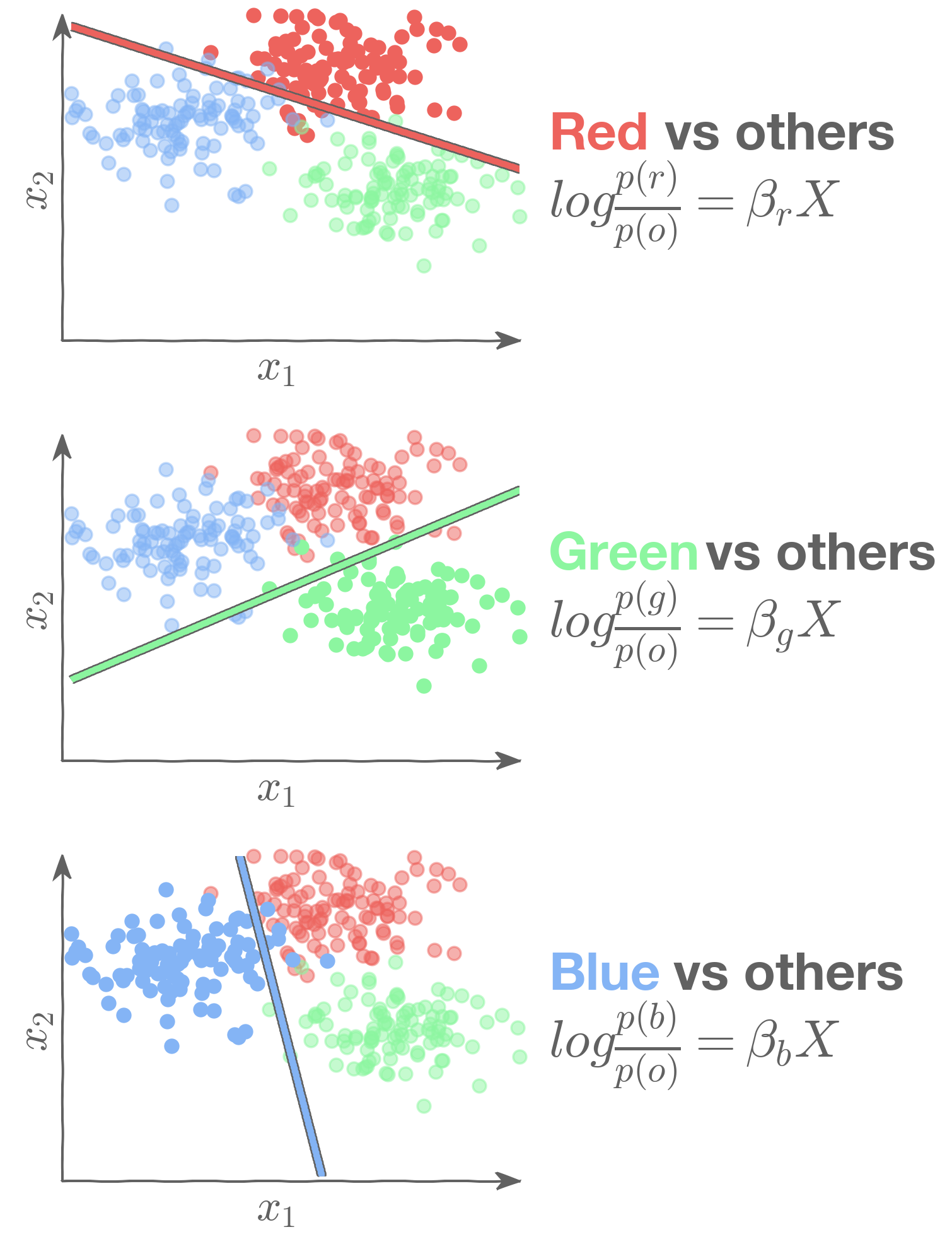
 Sklearn normalizes the output of each of the three models when predicting probabilities:

1.3 True Multinomial Logistic Regression

Another option for a multiclass logistic regression model is what we will call the "true" multinomial logistic regression model. Here one of the classes is chosen as the baseline group (think  group in typical logistic regression), and the other  classes are compared to it. Thus, a sequence of  binary models are built to predict being in class  as opposed to the baseline class.

This is mathematically equivalent to using the softmax function:

And the cross-entropy as the loss function:

1.4 Comparing OVR and true multinomial logistic regression

True Multinomial is slightly more efficient in estimation since there are technically fewer parameters (though sklearn reports extra ones to normalize the calculations to 1) and it is more suitable for inferences/group comparisons.

OVR is often preferred for determining classification: you simply just predict from all 3 separate models (for each individual observation) and choose the highest probability.

They give VERY similar results in estimated probabilities and classifications.

1.5 Motivation

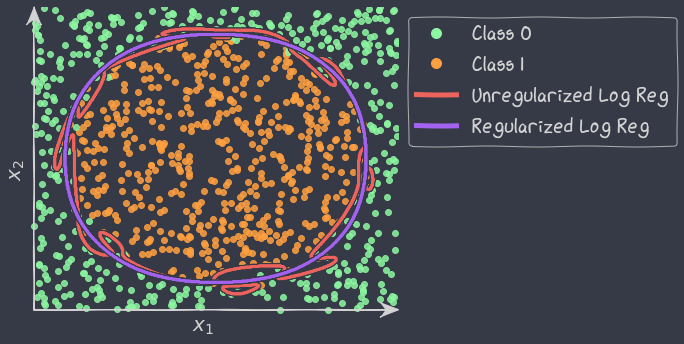
The problem of separation arises when the binary responses can be separated into all 0s and all 1s as a linear function of the predictors, as in the image below.

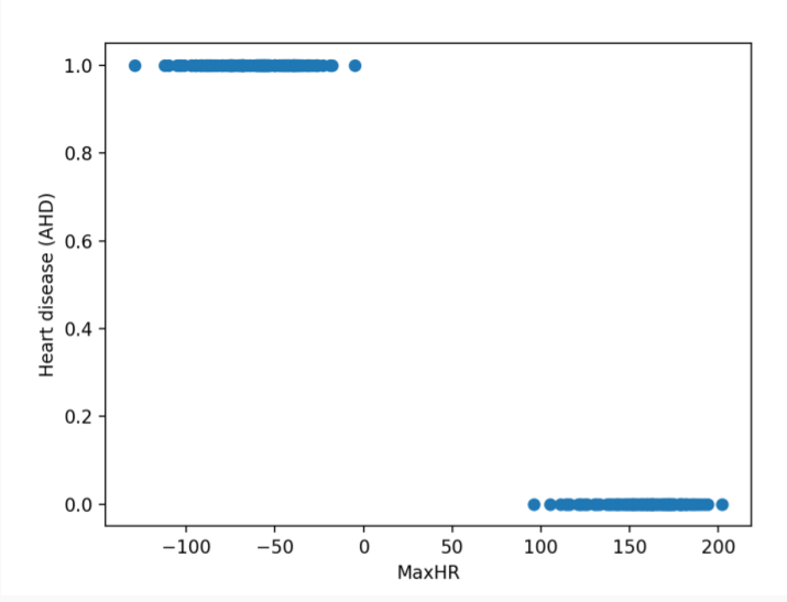
The Maximum Likelihood Estimation (MLE) does not exist when the data is perfectly separable. The likelihood always increases with the magnitude of the estimated coefficients. To solve this issue, we need to use regularization.

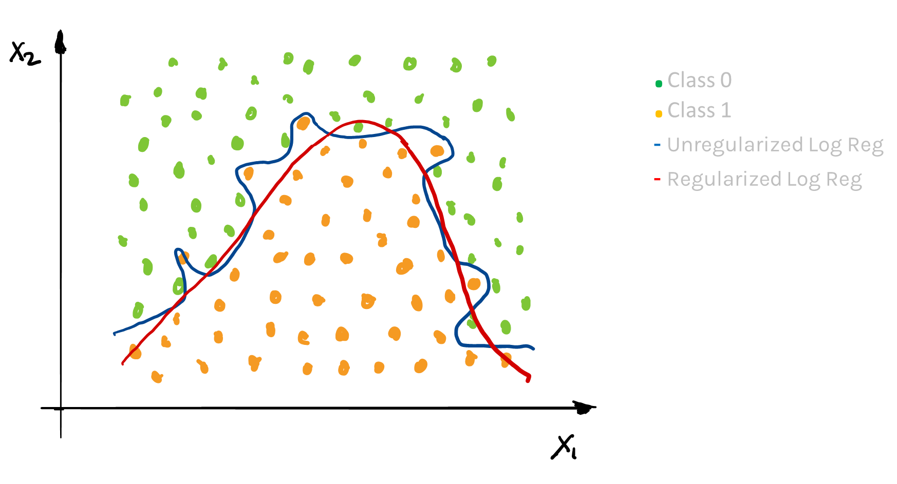
1.6 Regularization in Logistic Regression

Based on the Likelihood framework, a loss function can be determined based on the log-likelihood function. We saw in linear regression that maximizing the log-likelihood is equivalent to minimizing the sum of squares.

And a regularization approach was to add a penalty factor to this equation, which for Ridge Regression becomes:

Note: this penalty shrinks the estimates towards zero, and has the analogue of using a Normal prior centered at zero in the Bayesian paradigm.

A similar approach can be used in logistic regression. Here, maximizing the log-likelihood is equivalent to minimizing the following loss function:

where

A penalty factor can then be added to this loss function and results in a new loss function that penalizes large values of the parameters:

The result is just like in linear regression: it shrinks the parameter estimates towards zero. In practice, the intercept is usually not part of the penalty factor. Note: the sklearn package uses a different tuning parameter: instead of  they use a constant that is essentially .

Just like in linear regression, the shrinkage factor must be chosen. Through building multiple training and test sets (cross-validation), we can select the best shrinkage factor to mimic out-of-sample prediction.

2. Missingness

In all of the datasets we've looked at so far, every observation has always had a recorded value for each predictor variable as well as the response. That is, there were no missing values. But in the real world we are usually not so lucky. Missing data can arise in many ways. For example:

• A survey was conducted, and some values were just randomly missed when being entered in the computer
• Someone completing a survey chooses not to respond to a question like, "Have you ever used illegal drugs?"
• You decide to start collecting a new variable partway through the data collection of a study
• You want to measure the speed of meteors, and some of them are just ‘too quick’ to be measured properly

In what ways are some of the examples above similar? How do they differ? We'll find it useful to categorize all instances of missingness into 3 major types:

2.1 Missing Completely at Random (MCAR)

For this scenario, the probability of missingness is the same for every observation. This would be like randomly poking holes in a data set. Examples:

• A coin is flipped to determine whether an entry is removed.
• Values were just randomly missed when being entered in the computer.

This is the best-case scenario for missingness, and the easiest to handle. Because the missingness does not depend on any other predictors, either included in our data or not, we can simply remove (or 'drop') observations with missing values. This would be equivalent to removing a random subset of the data, which should not bias the remaining dataset toward observations of a certain kind. This should then have no effect on our inference (that is, the estimate of the betas).

Inserting or 'imputing' predictions for the missing values is also an option and will be discussed in more detail below.

2.2 Missing at Random (MAR)

For this scenario, the probability of missingness depends only on available information (in other predictors). While less ideal than MCAR, MAR is still a case that can be handled.

An example for MAR would be men and women responding at different rates to the question, "have you ever been harassed at work?"In this hypothetical example let's assume that women were more likely than men to leave the question about harassment blank. In this scenario, dropping observations with this response missing would bias our data as we would drop more women than men.

Effect if you ignore: inferences (estimates of the 's) are biased and predictions are usually worsened.

How to handle: use the values in the other predictors to build a model to impute values for the missing entries.

2.3 Missing Not at Random (MNAR)

For this scenario, the probability of missingness depends on information that has not been recorded. Missing Not at Random is the worst-case scenario, and impossible to resolve. Some examples are:

• Patients drop out of a study because they experience some really bad side effect that was not measured.
• Cheaters are less likely to respond when asked if they've ever cheated.

Effect if you ignore: inferences (estimates of betas) become biased, and predictions are usually worsened.

How to handle: you can attempt to 'improve' things with an imputation method similar to that recommended for MAR, but you may never completely fix the bias.

The bad news is that we can never be certain about what type of missingness we are dealing with by inspecting the data. Generally, it cannot be determined whether data are missing completely at random (MCAR) or whether the missingness depends on unobserved predictors or the missing data themselves (MNAR). The problem is that these potential “lurking variables” are unobserved (by definition) and so can never be completely ruled out.

In practice, a model with as many predictors as possible is used so that the ‘missing at random’ (MAR) assumption is reasonable.

2.4 Identifying and Handling Missingness

The first step to addressing missingness is to recognize it in your data.

So, what does missingness look like in a Pandas DataFrame? Pandas uses NumPy’s special NaN datatype to denote missing values. It is also common to see the None type used to signify a missing value.

Pandas has a helpful method to quickly discover missingness in your DataFrame. The isna() method will return a boolean matrix with True in each index that had either NaN or None and False everywhere else.

This boolean matrix can be used for selecting just those indices that have missing values. Or, if you use the negation operator, you can select just those indices without missingness.

You will need to resolve the missingness before you can fit an SKLearn model like LinearRegression on your data. So how do we resolve the missingness?

Option 1: Dropping

The simplest ways to handle missing data it is by just throwing away or ‘dropping’ the observations that have any missing values.
Pandas dropna(axis=0,1) will drop any rows or columns with one or more missing values from your Pandas DataFrame.
Dropping is ‘easy,’ but when is it advisable?

It is probably a good idea to drop a predictor column if it is missing large proportion of observations.

Similarly, if a given observation row has many missing values, then we might want to drop it as well.

But dropping rows can have negative consequences, and not just because we are throwing away data! If the observations with missing values differ systematically from observations without missing values, then we risk biasing our dataset by dropping rows or columns with missingness! That is, if certain values are not missing completely at random but for some underlying reason, or, if the missingness is itself correlated with some other predictors of an observation, then dropping such rows can get us into trouble. These are the MAR and MNAR cases we spoke about earlier.

Option 2: Imputation

Rather than simply dropping missing values, we could try to fill them in with well chosen values. This ‘filling in’ is called ‘imputation.’ The hope is that this will allow us to retain the relevant information in observations with missingness. Dropping would have just thrown it away!

Simple Imputation Methods

A common method is to impute using some sort of average value. What we mean by ‘average’ can depend on the type of the predictor variable we want to impute:

• Quantitative: Impute the mean or median value
• Categorical: Impute the mode, that is, the most common class

Imputing average values is easy in Pandas. First, calculate the average value you wish to impute. For example, the mean. Next, use the fillna() method on the column with the missingness you want to fill and pass the value to impute as an argument.
Let’s see an example!

df['x1'].fillna(df['x1'].mean())

This code first calculates the mean of the column x1. Note the mean method ignores any missing values in the calculation. It then fills all missing values in x1 with this mean!

Imputation Example

Here’s a visual explanation for imputation for a dataset with two predictors: X1, which is quantitative, and X2, which is categorical

X1	X2
10	.
5	1
21	0
15	0
16	.
.	.
21	1
12	0
.	0

For X1 we can replace its missing values by imputing with the column’s mean value.

For X2 we can impute using its mode, or most common value (i.e., mode).

Let's call these new predictors with the imputed values  and . Now, we could proceed with  and  as our only 2 predictors. But doing so would in effect be throwing away some potentially useful information.

What information could that be? The fact that these values were originally missing!

2.5 Missingness Indicator Variable

We can capture the fact that a value was missing by creating 2 new indicator variables.

For example, the indicator variable , takes the value 1 for all rows where  originally had a missing value, and 0 otherwise.

Similarly,, takes the value 1 for all rows where  originally had a missing value, and 0 otherwise.

10	.	0	1
5	1	0	0
21	0	0	0
15	0	0	0
16	.	0	1
.	.	1	1
21	1	0	0
12	0	0	0
.	0	1	0

Our final design matrix would then be:

•  - continuous variable with mean imputation
•  - categorical variable with mode imputation
•  - indicating previously missing values in the continuous variable 
•  - indicating previously missing values in the categorical variable 

Why Use a Missingness Indicator Variable?

Q: How does this missingness indicator variable improve the model?

A: Because the group of observations with a missing entry may be systematically different than those with the variable measured.

Treating them equivalently could lead to bias in quantifying relationships (the s) and underperformance in prediction.

Example: Imagine a survey question that asks whether or not someone has ever recreationally used opioids, and some people chose not to respond.

Does the fact that they did not respond itself provide extra information? Should we treat them equivalently as never-users?

This approach essentially creates a third group for this predictor: the “did not respond” group.

2.6 Model-Based Imputation

With simple imputation, we were only using information about the particular predictor we wanted to perform the imputation on. But each observation may have many other predictors, and these other predictors may be related to the missing predictor!

Model-Based imputation uses information contained in the other predictors to help us learn a value to impute.

Here we have two predictors,  and .

red-orange	1
orange	?
gold	0.5
yellow	0.1
green-yellow	?
green	10
teal	0.03

How can we use a model to fill in the missing values in ?

Think of  as the predictor and  as the response. An imputation model can then learn the relationship between  and  from those observations with no missingness.

2.6 kNN Imputation

kNN is perhaps the simplest model-based imputation method. Let's see a kNN imputation model in action with k=2.

To impute a missing value, find the missing observation's 2 nearest neighbors in terms of the data we do have (that is,  ). We only consider observations without missingness as potential neighbors.We then average these neighbors' values for the missing predictor and impute! You can repeat this process for each observation that needs imputation.

red-orange	1
orange	0.75 = (1 + 0.5) / 2
gold	0.5
yellow	0.1
green-yellow	5.05 = (10 + 0.1) / 2
green	10
teal	0.03

2.7 Different Imputation Models

We can use all kinds of models as imputers:

• A regression model for imputing continuous variables
• A classification model for imputing categorical variables

The trick is to treat the column to be imputed as a new response variable.