（10-2-01）TensorFlow深度信念网络实战：深度信念网络应用实战：程序缺陷预测(1)

10.2  深度信念网络应用实战：程序缺陷预测

经过本章前面内容的学习，已经基本了解了深度信念网络的基础知识。在本节的内容中，将通过具体实例的实现过程，详细讲解在在TensorFlow中使用深度信念网络的方法。本实例的功能是，使用 DBN 模型分别进行ANN、LogisticRegression、GaussianNB 和 RandomForestClassifier 的训练和集成，用于在有缺陷的代码和干净的代码之间进行分类。本项目程程序保存在ipynb文件中，将在谷歌的Colaboratory中调试运行。

10.2.1  使用DBN模型进行ANN处理

ANN是人工神经网络（Artificial Neural Network）的简称，是指由大量的处理单元(神经元) 互相连接而形成的复杂网络结构，是对人脑组织结构和运行机制的某种抽象、简化和模拟。以数学模型模拟神经元活动，是基于模仿大脑神经网络结构和功能而建立的一种信息处理系统。编写文件JustInTime_SW_Pred_v1.ipynb使用DBN模型进行ANN处理，具体实现流程如下：

（1）导入谷歌的库colab，查看驱动器的位置，代码如下：

from google.colab import drive
drive.mount('/content/drive/')

执行后会输出：

Drive already mounted at /content/drive/; to attempt to forcibly remount, call drive.mount("/content/drive/", force_remount=True).

（2）导入需要用到的库，代码如下：

import tensorflow as tf
import sklearn.metrics
from sklearn.metrics import log_loss, accuracy_score
import numpy as np
import pandas as pd
import matplotlib.pyplot as plt

（3）导入CSV文件，并获取文件中的数据数目，代码如下：

df= pd.read_csv('/content/drive/My Drive/dataset/bugzilla.csv')
def normalize(x):
  x = x.astype(float)
  min = np.min(x)
  max = np.max(x)
  return (x - min)/(max-min)

def view_values(X, y, example):
    label = y.loc[example]
    image = X.loc[example,:].values.reshape([-1,1])
    print(image)

print("Shape of dataframe: ", df.shape)   #train

执行后会输出：

Shape of dataframe:  (4620, 17)

（4）查看前5行数据中的信息，代码如下：

df.head()

执行后会输出：

class RBM(object):
    
    def __init__(self, input_size, output_size, 
                 learning_rate, epochs, batchsize):
        #定义超参数
        self._input_size = input_size
        self._output_size = output_size
        self.learning_rate = learning_rate
        self.epochs = epochs
        self.batchsize = batchsize
        
        #使用零矩阵初始化权重和偏差
        self.w = np.zeros([input_size, output_size], dtype=np.float32)
        self.hb = np.zeros([output_size], dtype=np.float32)
        self.vb = np.zeros([input_size], dtype=np.float32)

（5）创建受限玻尔兹曼机类RBM，然后定义需要的超参数，代码如下：

    #向前传递
    def prob_h_given_v(self, visible, w, hb):
        return tf.nn.sigmoid(tf.matmul(visible, w) + hb)
    #向后传递
    def prob_v_given_h(self, hidden, w, vb):
        return tf.nn.sigmoid(tf.matmul(hidden, tf.transpose(w)) + vb)
    #采样函数
    def sample_prob(self, probs):
        return tf.nn.relu(tf.sign(probs - tf.random_uniform(tf.shape(probs))))

（6）分别创建向前传递函数、向后传递函数和采样函数，其中h为隐藏层，v为可见层。代码如下：

    #向前传递

    def prob_h_given_v(self, visible, w, hb):

        return tf.nn.sigmoid(tf.matmul(visible, w) + hb)

    #向后传递

    def prob_v_given_h(self, hidden, w, vb):

        return tf.nn.sigmoid(tf.matmul(hidden, tf.transpose(w)) + vb)

    #采样函数

    def sample_prob(self, probs):

        return tf.nn.relu(tf.sign(probs - tf.random_uniform(tf.shape(probs))))

（7）创建训练函数train()，为了在训练时更新权重，我们设置执行收缩发散功能，并将误差定义为MSE（均方误差）。代码如下：

    def train(self, X):
        _w = tf.placeholder(tf.float32, [self._input_size, self._output_size])
        _hb = tf.placeholder(tf.float32, [self._output_size])
        _vb = tf.placeholder(tf.float32, [self._input_size])
        
        prv_w = np.zeros([self._input_size, self._output_size], dtype=np.float32)
        prv_hb = np.zeros([self._output_size], dtype=np.float32)
        prv_vb = np.zeros([self._input_size], dtype=np.float32)
        
        cur_w = np.zeros([self._input_size, self._output_size], dtype=np.float32)
        cur_hb = np.zeros([self._output_size], dtype=np.float32)
        cur_vb = np.zeros([self._input_size], dtype=np.float32)
        v0 = tf.placeholder(tf.float32, [None, self._input_size])
        h0 = self.sample_prob(self.prob_h_given_v(v0, _w, _hb))
        v1 = self.sample_prob(self.prob_v_given_h(h0, _w, _vb))
        h1 = self.prob_h_given_v(v1, _w, _hb)
      
        positive_grad = tf.matmul(tf.transpose(v0), h0)
        negative_grad = tf.matmul(tf.transpose(v1), h1)
        
        update_w = _w + self.learning_rate * (positive_grad - negative_grad) / tf.to_float(tf.shape(v0)[0])
        update_vb = _vb +  self.learning_rate * tf.reduce_mean(v0 - v1, 0)
        update_hb = _hb +  self.learning_rate * tf.reduce_mean(h0 - h1, 0)
        #还将误差定义为MSE
        err = tf.reduce_mean(tf.square(v0 - v1))
        
        error_list = []

        with tf.Session() as sess:
            sess.run(tf.global_variables_initializer())
            
            for epoch in range(self.epochs):
                for start, end in zip(range(0, len(X),  self.batchsize),range(self.batchsize,len(X), self.batchsize)):
                    batch = X[start:end]
                    cur_w = sess.run(update_w, feed_dict={v0: batch, _w: prv_w, _hb: prv_hb, _vb: prv_vb})
                    cur_hb = sess.run(update_hb, feed_dict={v0: batch,  _w: prv_w, _hb: prv_hb, _vb: prv_vb})
                    cur_vb = sess.run(update_vb, feed_dict={v0: batch, _w: prv_w, _hb: prv_hb, _vb: prv_vb})
                    prv_w = cur_w
                    prv_hb = cur_hb
                    prv_vb = cur_vb
                error = sess.run(err, feed_dict={v0: X, _w: cur_w, _vb: cur_vb, _hb: cur_hb})
                print ('Epoch: %d' % epoch,'reconstruction error: %f' % error)
                error_list.append(error)
            self.w = prv_w
            self.hb = prv_hb
            self.vb = prv_vb
            return error_list

（8）编写函数rbm_output()，功能是从RBM已学习的生成模型生成新特征。代码如下：

    def rbm_output(self, X):
        
        input_X = tf.constant(X)
        _w = tf.constant(self.w)
        _hb = tf.constant(self.hb)
        _vb = tf.constant(self.vb)
        out = tf.nn.sigmoid(tf.matmul(input_X, _w) + _hb)
        hiddenGen = self.sample_prob(self.prob_h_given_v(input_X, _w, _hb))
        visibleGen = self.sample_prob(self.prob_v_given_h(hiddenGen, _w, _vb))
        with tf.Session() as sess:
            sess.run(tf.global_variables_initializer())
            return sess.run(out), sess.run(visibleGen), sess.run(hiddenGen)

（9）开始进行训练，为了实现更平衡的数据帧，使用函数drop()删除不必要的字符串列。代码如下：

deleted = 0
for i in range(0, df.shape[0]-1):
  if deleted == 1230:
    break
  elif df.iloc[i].bug == 0:
    df = df.drop(df.index[i])
    deleted = deleted + 1

#删除不必要的字符串列
df = df.drop(['commitdate','transactionid'], axis=1)

#分割df
train_X = df.iloc[:,:-1].apply(func=normalize, axis=0)
train_Y = df.iloc[:,-1]

# df=df.drop(['transactionid'], axis=1)
print(df.head())

执行后会输出：

   ns  nm  nf   entropy        la  ...       npt  exp    rexp  sexp  bug
0   1   1   3  0.579380  0.093620  ...  0.666667  143  133.50   129    1
1   1   1   1  0.000000  0.000000  ...  1.000000  140  140.00   137    1
3   1   1   8  0.685328  0.016039  ...  1.000000  579  479.25   550    0
5   1   1  16  0.760777  0.018308  ...  0.750000  595  495.25   566    0
7   2   2  33  0.816160  0.095682  ...  0.727273  482  382.25   474    0

[5 rows x 15 columns]

（10）在训练时设置限制玻尔兹曼机的参数，代码如下：

import tensorflow.compat.v1 as tf
tf.disable_v2_behavior()

outputList = []
error_list = []

#遍历每个RBM输入输出列表
for i in range(0, len(rbm_list)):
    print('RBM', i+1)
    #训练新的RBM
    rbm = rbm_list[i]
    err = rbm.train(inputX)
    error_list.append(err)

    #返回输出层
    #sess.run(out), sess.run(visibleGen), sess.run(hiddenGen)
    outputX, reconstructedX, hiddenX = rbm.rbm_output(inputX)
    outputList.append(outputX)
    inputX= hiddenX

执行后会输出：

deprecated and will be removed in a future version.
Instructions for updating:
Use `tf.cast` instead.
Epoch: 0 reconstruction error: 0.113313
Epoch: 1 reconstruction error: 0.117359
Epoch: 2 reconstruction error: 0.114953
Epoch: 3 reconstruction error: 0.111951
Epoch: 4 reconstruction error: 0.110032
Epoch: 5 reconstruction error: 0.111399
Epoch: 6 reconstruction error: 0.111426
Epoch: 7 reconstruction error: 0.108291
Epoch: 8 reconstruction error: 0.109852
Epoch: 9 reconstruction error: 0.107341
Epoch: 10 reconstruction error: 0.103858
Epoch: 11 reconstruction error: 0.107152
Epoch: 12 reconstruction error: 0.108607
Epoch: 13 reconstruction error: 0.102160
Epoch: 14 reconstruction error: 0.106119
Epoch: 15 reconstruction error: 0.107382
Epoch: 16 reconstruction error: 0.108130
......
Epoch: 145 reconstruction error: 0.125590
Epoch: 146 reconstruction error: 0.122321
Epoch: 147 reconstruction error: 0.125713
Epoch: 148 reconstruction error: 0.127262
Epoch: 149 reconstruction error: 0.123992

（12）使用for循环遍历上面的每个RBM输入输出列表，并循环绘制重建误差和RBM的可视化图，代码如下：

i = 1
for err in error_list:
    print("RBM",i)
    pd.Series(err).plot(logy=False)
    plt.xlabel("Epoch")
    plt.ylabel("Reconstruction Error")
    plt.show()
    i += 1

执行效果如图10-6所示。

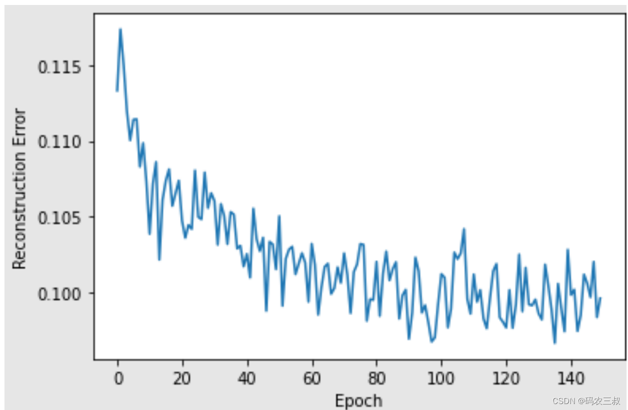
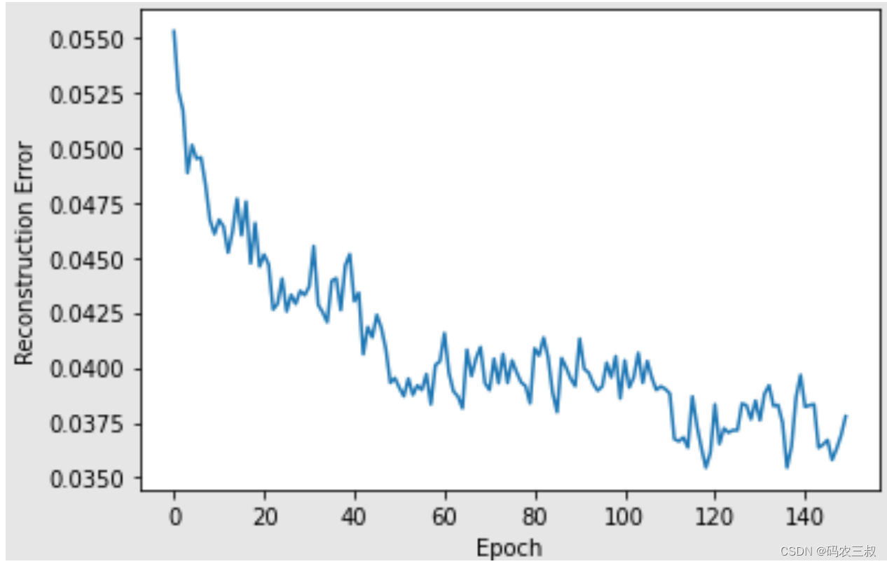
图10-6  可视化图