


论文地址:https://arxiv.org/pdf/2402.17764.pdf
相关博客
【自然语言处理】【大模型】BitNet:用1-bit Transformer训练LLM
【自然语言处理】BitNet b1.58:1bit LLM时代
【自然语言处理】【长文本处理】RMT:能处理长度超过一百万token的Transformer
【自然语言处理】【大模型】MPT模型结构源码解析(单机版)
【自然语言处理】【大模型】ChatGLM-6B模型结构代码解析(单机版)
【自然语言处理】【大模型】BLOOM模型结构源码解析(单机版)
一、BitNet
BitNet采用了与Transformer基本一致的模型架构,仅将标准矩阵乘法层换成了BitLinear,其他组件仍然是高精度的。BitLinear主要是包含的操纵:权重量化、激活量化以及LayerNorm。
权重量化。通过减均值实现0中心化,然后用sign实现二值化。假设全精度权重为
W
∈
R
n
×
m
W\in\mathcal{R}^{n\times m}
W∈Rn×m,则二值量化过程为
W
~
=
Sign
(
W
−
α
)
(1)
\widetilde{W}=\text{Sign}(W-\alpha) \tag{1} \\
W
=Sign(W−α)(1)
Sign ( W i j ) = { + 1 , if W i j > 0 − 1 , if W i j ≤ 0 (2) \text{Sign}(W_{ij})=\begin{cases} +1,&&\text{if}\;W_{ij}>0 \\ -1,&&\text{if}\;W_{ij}\leq 0 \\ \end{cases} \tag{2} \\ Sign(Wij)={+1,−1,ifWij>0ifWij≤0(2)
α = 1 n m ∑ i j W i j (3) \alpha=\frac{1}{nm}\sum_{ij}W_{ij} \tag{3} \\ α=nm1ij∑Wij(3)
激活量化。使用absmax的方式将激活量化至b-bit。具体的实现方式是乘以
Q
b
Q_b
Qb再除以输入矩阵的最大绝对值,从而将激活缩放至
[
−
Q
b
,
Q
b
]
(
Q
b
=
2
b
−
1
)
[-Q_b,Q_b](Q_b=2^{b-1})
[−Qb,Qb](Qb=2b−1),即
x
~
=
Quant
(
x
)
=
Clip
(
x
×
Q
b
γ
,
−
Q
b
+
ϵ
,
Q
b
−
ϵ
)
(4)
\tilde{x}=\text{Quant}(x)=\text{Clip}(x\times\frac{Q_b}{\gamma},-Q_b+\epsilon,Q_b-\epsilon) \tag{4}\\
x~=Quant(x)=Clip(x×γQb,−Qb+ϵ,Qb−ϵ)(4)
Clip ( x , a , b ) = max ( a , min ( b , x ) ) , γ = ∥ x ∥ ∞ (5) \text{Clip}(x,a,b)=\max(a,\min(b,x)),\quad\gamma=\parallel x\parallel_\infty \tag{5} \\ Clip(x,a,b)=max(a,min(b,x)),γ=∥x∥∞(5)
其中 ϵ \epsilon ϵ是防止裁剪时溢出的小浮点数。
对于非线性函数之前的激活值则采用不同的量化方式,通过减轻最小值的方式将其缩放至
[
0
,
Q
b
]
[0,Q_b]
[0,Qb],从而保证所有值均为非负:
x
~
=
Quant
(
x
)
=
Clip
(
(
x
−
η
)
×
Q
b
γ
,
ϵ
,
Q
b
−
ϵ
)
,
η
=
min
i
,
j
x
i
j
(6)
\tilde{x}=\text{Quant}(x)=\text{Clip}((x-\eta)\times\frac{Q_b}{\gamma},\epsilon,Q_b-\epsilon),\quad\eta=\min_{i,j}x_{ij}\tag{6} \\
x~=Quant(x)=Clip((x−η)×γQb,ϵ,Qb−ϵ),η=i,jminxij(6)
LayerNorm。在对激活值量化前,为了保证量化后的方差稳定,采用了SubLN。
BitLinear的完成计算过程为
y
=
W
~
x
~
=
W
~
Quant
(
LN
(
x
)
)
×
β
γ
Q
b
(7)
y=\widetilde{W}\tilde{x}=\widetilde{W}\text{Quant}(\text{LN}(x))\times\frac{\beta\gamma}{Q_b}\tag{7} \\
y=W
x~=W
Quant(LN(x))×Qbβγ(7)
LN ( x ) = x − E ( x ) Var ( x ) + ϵ , β = 1 n m ∥ W ∥ 1 (8) \text{LN}(x)=\frac{x-E(x)}{\sqrt{\text{Var}(x)+\epsilon}},\quad\beta=\frac{1}{nm}\parallel W\parallel_1 \tag{8} \\ LN(x)=Var(x)+ϵx−E(x),β=nm1∥W∥1(8)
二、BitNet b1.58
BitNet b1.58在BitNet的基础上做了一些修改。
权重量化。采用absmean的方式将权重约束在
{
−
1
,
0
,
1
}
\{-1,0,1\}
{−1,0,1}中,而BitNet则将权重约束为二值
{
−
1
,
1
}
\{-1,1\}
{−1,1}。具体来说,先使用平均绝对值来缩放权重,然后通过舍入的方式转换为
{
−
1
,
0
,
1
}
\{-1,0,1\}
{−1,0,1}:
W
~
=
RoundClip
(
W
γ
+
ϵ
,
−
1
,
1
)
(9)
\widetilde{W}=\text{RoundClip}(\frac{W}{\gamma+\epsilon},-1,1)\tag{9} \\
W
=RoundClip(γ+ϵW,−1,1)(9)
RoundClip ( x , a , b ) = max ( a , min ( b , round ( x ) ) ) (10) \text{RoundClip}(x,a,b)=\max(a,\min(b,\text{round}(x)))\tag{10} \\ RoundClip(x,a,b)=max(a,min(b,round(x)))(10)
γ = 1 n m ∑ i j ∣ W i j ∣ (11) \gamma=\frac{1}{nm}\sum_{ij}|W_{ij}|\tag{11} \\ γ=nm1ij∑∣Wij∣(11)
激活量化。同BitNet一样,但是对于非线性函数前的激活不再量化至 [ 0 , Q b ] [0,Q_b] [0,Qb],而是都量化至 [ − Q b , Q b ] [-Q_b,Q_b] [−Qb,Qb]。
此外,为了能够方便于开源软件兼容,整体结构采用类似LLaMA的结构。具体来说,使用RMSNorm、SwiGLU、RoPE并移除所有偏置。
三、实验
1. 困惑度
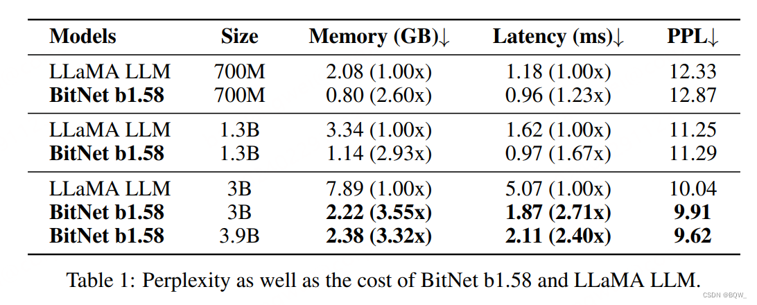
BitNet b1.58在3B大小时,困惑度与LLaMA相匹配,但是速度快2.71倍且显存使用减少3.55倍。当BitNet b1.58大小为3.9B时,速度快2.4倍且显存减少3.32倍,并且效果显著优于LLaMA 3B。
2. 下游任务
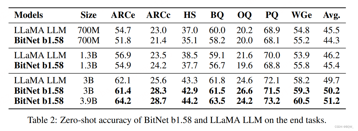
随着模型尺寸的增加,BitNet b1.58和LLaMA在下游任务上的差距逐步缩小。在尺寸达到3B时,BitNet b.158能够与全精度相匹配。
3. 显存和延时
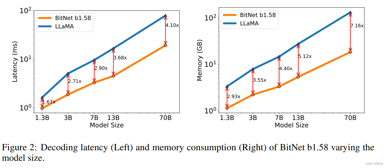
随着模型尺寸的增加,BitNet b1.58的速度优势和显存优势会更加明显。
4. 能耗
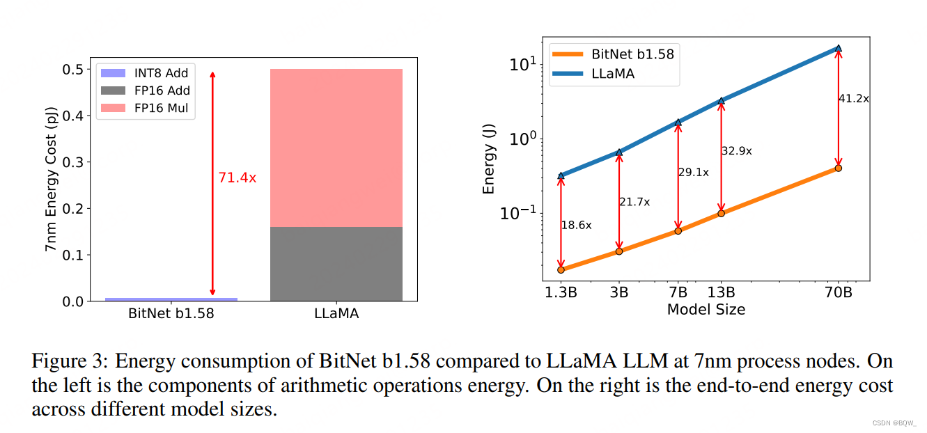
矩阵乘法是LLM中能耗最高的部分。BitNet b1.58主要是INT8的加法计算,而LLaMA则是由FP16加法和乘法组成。在7nm芯片上,BitNet b1.58能够节约71.4倍的计算能耗。随着模型尺寸的增加,BitNet b1.58在能耗方面会越来越高效。
5. 吞吐
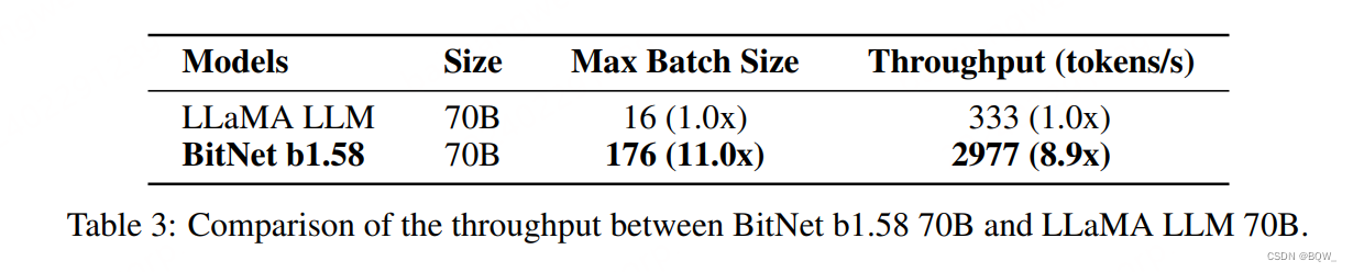
相同机器下,BitNet b1.58的batch size是LLaMA LLM的11倍,吞吐则是8.9倍。


 1201
1201

 被折叠的 条评论
为什么被折叠?
被折叠的 条评论
为什么被折叠?
 到【灌水乐园】发言


