5.深度学习练习：Deep Neural Network for Image Classification: Application

本文节选自吴恩达老师《深度学习专项课程》编程作业，在此表示感谢。

课程链接：https://www.deeplearning.ai/deep-learning-specialization/

After this assignment you will be able to:

• Build and apply a deep neural network to supervised learning.

---

目录

1 - Packages

2 - Dataset

3 - Architecture of your model

3.1 - 2-layer neural network

3.2 - L-layer deep neural network

3.3 - General methodology

4 - Two-layer neural network

5 - L-layer Neural Network

6) Results Analysis

7) Test with your own image (optional/ungraded exercise)

---

1 - Packages

Let's first import all the packages that you will need during this assignment.

• numpy is the fundamental package for scientific computing with Python.
• matplotlib is a library to plot graphs in Python.
• h5py is a common package to interact with a dataset that is stored on an H5 file.
• PIL and scipy are used here to test your model with your own picture at the end.
• dnn_app_utils provides the functions implemented in the "Building your Deep Neural Network: Step by Step" assignment to this notebook.

import time
import numpy as np
import h5py
import matplotlib.pyplot as plt
import scipy
from PIL import Image
from scipy import ndimage
from dnn_app_utils_v2 import *

%matplotlib inline
plt.rcParams['figure.figsize'] = (5.0, 4.0) # set default size of plots
plt.rcParams['image.interpolation'] = 'nearest'
plt.rcParams['image.cmap'] = 'gray'

%load_ext autoreload
%autoreload 2

np.random.seed(1)

---

2 - Dataset

You will use the same "Cat vs non-Cat" dataset as in "Logistic Regression as a Neural Network" (Assignment 2). The model you had built had 70% test accuracy on classifying cats vs non-cats images. Hopefully, your new model will perform a better!

Problem Statement: You are given a dataset ("data.h5") containing:

- a training set of m_train images labelled as cat (1) or non-cat (0)
- a test set of m_test images labelled as cat and non-cat
- each image is of shape (num_px, num_px, 3) where 3 is for the 3 channels (RGB).

Let's get more familiar with the dataset. Load the data by running the cell belo

train_x_orig, train_y, test_x_orig, test_y, classes = load_data()

# Example of a picture
index = 9
plt.imshow(train_x_orig[index])
print ("y = " + str(train_y[0,index]) + ". It's a " + classes[train_y[0,index]].decode("utf-8") +  " picture.")
print(train_x_orig.shape)

As usual, you reshape and standardize the images before feeding them to the network. The code is given in the cell below.

# Reshape the training and test examples 
train_x_flatten = train_x_orig.reshape(train_x_orig.shape[0], -1).T   # The "-1" makes reshape flatten the remaining dimensions
test_x_flatten = test_x_orig.reshape(test_x_orig.shape[0], -1).T

# Standardize data to have feature values between 0 and 1.
train_x = train_x_flatten/255.
test_x = test_x_flatten/255.

print ("train_x's shape: " + str(train_x.shape))
print ("test_x's shape: " + str(test_x.shape))

---

3 - Architecture of your model

Now that you are familiar with the dataset, it is time to build a deep neural network to distinguish cat images from non-cat images.

You will build two different models:

• A 2-layer neural network
• An L-layer deep neural network

You will then compare the performance of these models, and also try out different values for ?L.

Let's look at the two architectures.

3.1 - 2-layer neural network

The model can be summarized as: ***INPUT -> LINEAR -> RELU -> LINEAR -> SIGMOID -> OUTPUT***.

3.2 - L-layer deep neural network

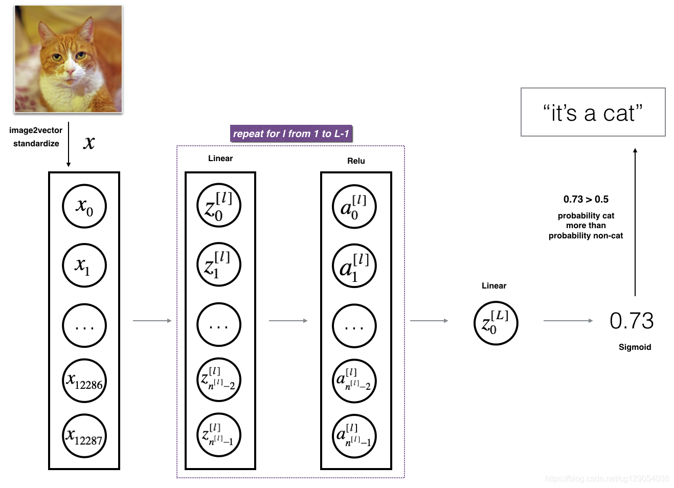
The model can be summarized as: ***[LINEAR -> RELU] ×× (L-1) -> LINEAR -> SIGMOID***

3.3 - General methodology

As usual you will follow the Deep Learning methodology to build the model:

1. Initialize parameters / Define hyperparameters
2. Loop for num_iterations:
    a. Forward propagation
    b. Compute cost function
    c. Backward propagation
    d. Update parameters (using parameters, and grads from backprop) 
4. Use trained parameters to predict labels

---

4 - Two-layer neural network

Question: Use the helper functions you have implemented in the previous assignment to build a 2-layer neural network with the following structure: LINEAR -> RELU -> LINEAR -> SIGMOID. The functions you may need and their inputs are:

def initialize_parameters(n_x, n_h, n_y):
    ...
    return parameters 
def linear_activation_forward(A_prev, W, b, activation):
    ...
    return A, cache
def compute_cost(AL, Y):
    ...
    return cost
def linear_activation_backward(dA, cache, activation):
    ...
    return dA_prev, dW, db
def update_parameters(parameters, grads, learning_rate):
    ...
    return parameters

### CONSTANTS DEFINING THE MODEL ####
n_x = 12288     # num_px * num_px * 3
n_h = 7
n_y = 1
layers_dims = (n_x, n_h, n_y)

def two_layer_model(X, Y, layers_dims, learning_rate = 0.0075, num_iterations = 3000, print_cost=False):
    """
    Implements a two-layer neural network: LINEAR->RELU->LINEAR->SIGMOID.
    
    Arguments:
    X -- input data, of shape (n_x, number of examples)
    Y -- true "label" vector (containing 0 if cat, 1 if non-cat), of shape (1, number of examples)
    layers_dims -- dimensions of the layers (n_x, n_h, n_y)
    num_iterations -- number of iterations of the optimization loop
    learning_rate -- learning rate of the gradient descent update rule
    print_cost -- If set to True, this will print the cost every 100 iterations 
    
    Returns:
    parameters -- a dictionary containing W1, W2, b1, and b2
    """
    
    np.random.seed(1)
    grads = {}
    costs = []                              # to keep track of the cost
    m = X.shape[1]                           # number of examples
    (n_x, n_h, n_y) = layers_dims
    
    # Initialize parameters dictionary, by calling one of the functions you'd previously implemented
 
    parameters = initialize_parameters(n_x, n_h, n_y)
    
    # Get W1, b1, W2 and b2 from the dictionary parameters.
    W1 = parameters["W1"]
    b1 = parameters["b1"]
    W2 = parameters["W2"]
    b2 = parameters["b2"]
    
    # Loop (gradient descent)

    for i in range(0, num_iterations):

        # Forward propagation: LINEAR -> RELU -> LINEAR -> SIGMOID. Inputs: "X, W1, b1". Output: "A1, cache1, A2, cache2".
     
        A1, cache1 = linear_activation_forward(X, W1, b1, 'relu')
        A2, cache2 = linear_activation_forward(A1, W2, b2, 'sigmoid')
    
        cost = compute_cost(A2, Y)
      
        
        # Initializing backward propagation
        dA2 = - (np.divide(Y, A2) - np.divide(1 - Y, 1 - A2))
        
        # Backward propagation. Inputs: "dA2, cache2, cache1". Outputs: "dA1, dW2, db2; also dA0 (not used), dW1, db1".
      
        dA1, dW2, db2 = linear_activation_backward(dA2, cache2, 'sigmoid')
        dA0, dW1, db1 = linear_activation_backward(dA1, cache1, 'relu')
      
        
        # Set grads['dWl'] to dW1, grads['db1'] to db1, grads['dW2'] to dW2, grads['db2'] to db2
        grads['dW1'] = dW1
        grads['db1'] = db1
        grads['dW2'] = dW2
        grads['db2'] = db2
        
    
        parameters = update_parameters(parameters, grads, learning_rate = 0.0075)
 
        # Retrieve W1, b1, W2, b2 from parameters
        W1 = parameters["W1"]
        b1 = parameters["b1"]
        W2 = parameters["W2"]
        b2 = parameters["b2"]
        
        # Print the cost every 100 training example
        if print_cost and i % 100 == 0:
            print("Cost after iteration {}: {}".format(i, np.squeeze(cost)))
        if print_cost and i % 100 == 0:
            costs.append(cost)
       
    # plot the cost

    plt.plot(np.squeeze(costs))
    plt.ylabel('cost')
    plt.xlabel('iterations (per tens)')
    plt.title("Learning rate =" + str(learning_rate))
    plt.show()
    
    return parameters

parameters = two_layer_model(train_x, train_y, layers_dims = (n_x, n_h, n_y), num_iterations = 2500, print_cost=True)

predictions_train = predict(train_x, train_y, parameters)

---

5 - L-layer Neural Network

Question: Use the helper functions you have implemented previously to build an ?L-layer neural network with the following structure: [LINEAR -> RELU]××(L-1) -> LINEAR -> SIGMOID. The functions you may need and their inputs are:

def initialize_parameters_deep(layer_dims):
    ...
    return parameters 
def L_model_forward(X, parameters):
    ...
    return AL, caches
def compute_cost(AL, Y):
    ...
    return cost
def L_model_backward(AL, Y, caches):
    ...
    return grads
def update_parameters(parameters, grads, learning_rate):
    ...
    return parameters

layers_dims = [12288, 20, 7, 5, 1] #  5-layer model

def L_layer_model(X, Y, layers_dims, learning_rate = 0.0075, num_iterations = 3000, print_cost=False):#lr was 0.009
    """
    Implements a L-layer neural network: [LINEAR->RELU]*(L-1)->LINEAR->SIGMOID.
    
    Arguments:
    X -- data, numpy array of shape (number of examples, num_px * num_px * 3)
    Y -- true "label" vector (containing 0 if cat, 1 if non-cat), of shape (1, number of examples)
    layers_dims -- list containing the input size and each layer size, of length (number of layers + 1).
    learning_rate -- learning rate of the gradient descent update rule
    num_iterations -- number of iterations of the optimization loop
    print_cost -- if True, it prints the cost every 100 steps
    
    Returns:
    parameters -- parameters learnt by the model. They can then be used to predict.
    """

    np.random.seed(1)
    costs = []                         # keep track of cost
    
  
    parameters = initialize_parameters_deep(layers_dims)
   
    # Loop (gradient descent)
    for i in range(0, num_iterations):

        # Forward propagation: [LINEAR -> RELU]*(L-1) -> LINEAR -> SIGMOID.
        AL, caches = L_model_forward(X, parameters)

        # Compute cost.
        cost = compute_cost(AL, Y)
       
        # Backward propagation.
      
        grads = L_model_backward(AL, Y, caches)
       
        # Update parameters.
        parameters = update_parameters(parameters, grads, learning_rate = 0.0075)
                
        # Print the cost every 100 training example
        if print_cost and i % 100 == 0:
            print ("Cost after iteration %i: %f" %(i, cost))
        if print_cost and i % 100 == 0:
            costs.append(cost)
            
    # plot the cost
    plt.plot(np.squeeze(costs))
    plt.ylabel('cost')
    plt.xlabel('iterations (per tens)')
    plt.title("Learning rate =" + str(learning_rate))
    plt.show()
    
    return parameters

---

6) Results Analysis

First, let's take a look at some images the L-layer model labeled incorrectly. This will show a few mislabeled images.

A few type of images the model tends to do poorly on include:

• Cat body in an unusual position
• Cat appears against a background of a similar color
• Unusual cat color and species
• Camera Angle
• Brightness of the picture
• Scale variation (cat is very large or small in image)

---

7) Test with your own image (optional/ungraded exercise)

Congratulations on finishing this assignment. You can use your own image and see the output of your model. To do that:

my_image = "my_image.jpg" # change this to the name of your image file 
my_label_y = [] # the true class of your image (1 -> cat, 0 -> non-cat)


fname = "images/" + my_image
image = np.array(ndimage.imread(fname, flatten=False))
my_image = scipy.misc.imresize(image, size=(num_px,num_px)).reshape((num_px*num_px*3,1))
my_predicted_image = predict(my_image, my_label_y, parameters)

plt.imshow(image)
print ("y = " + str(np.squeeze(my_predicted_image)) + ", your L-layer model predicts a \"" + classes[int(np.squeeze(my_predicted_image)),].decode("utf-8") +  "\" picture.")