计算机视觉知识点集锦

最新推荐文章于 2025-03-24 14:24:50 发布

瑾怀轩

最新推荐文章于 2025-03-24 14:24:50 发布

阅读量2.7k

点赞数

文章标签：算法面试 python 计算机视觉目标检测

本文链接：https://blog.csdn.net/ckq707718837/article/details/123881939

版权

面试资料专栏收录该内容

5 篇文章

订阅专栏

本文详细介绍了计算机视觉中的关键概念，包括IoU（交并比）及其变体，以及mAP（平均精度均值）的计算方法。IoU用于衡量目标检测框的重合度，常用于NMS和mAP的计算。mAP是评估检测算法性能的重要指标，涉及PR曲线和不同插值方法。此外，还讨论了候选区域、非极大抑制（NMS）的原理与变体，以及多种目标检测网络模型如Yolo、SSD、RetinaNet和Faster R-CNN的RPN网络。

摘要生成于 C知道，由 DeepSeek-R1 满血版支持，前往体验 >

一、IoU

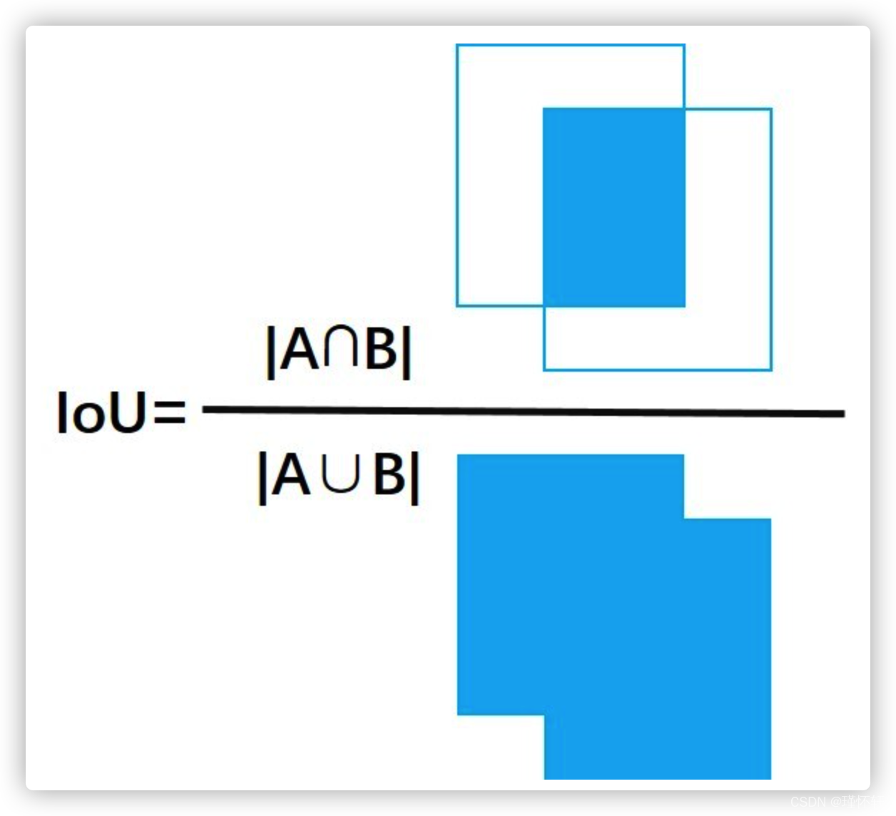
IoU 全称 intersection over Union ，交并比。主要用来衡量两个框重合程度。

计算公式： IoU = 两个框交集面积 / 两个框并集面积

例子：通常视觉任务中涉及真实框（标签框）、模型预测框（不止一个），通常通过它们重合程度进行判断预测的好不好，这也是Iou Loss 的核心思想。

主要应用在，候选区域、NMS 的去重，评估mAP，计算IoU Loss（这个也是描述框重合度的指标）

在处理多个proposals、pred bboxes时，由于预测的结果间可能存在高冗余（即同一个目标可能被预测多个矩形框），因此可以过滤掉一些彼此间高重合度的结果；

NMS：具体操作就是根据各个bbox的score降序排序，剔除与高score bbox有较高重合度的较低score bbox，那么重合度的度量指标就是IoU；（后面会详细讲）

mAP：得到检测算法的预测结果后，需要对pred bbox与gt bbox一起评估检测算法的性能，涉及到的评估指标为mAP，那么当一个pred bbox与gt bbox的重合度较高（如IoU score > 0.5），且分类结果也正确时，就可以认为是该pred bbox预测正确，这里也同样涉及到IoU的概念；

如何计算IoU,计算公式看似简单，但实现过程的复杂容易被忽视。

并集 = 两个框面积 - 交集面积。难点在于求交集。

首先想到根据两个框的相对位置分情形处理，那么来看看有多少种可能。

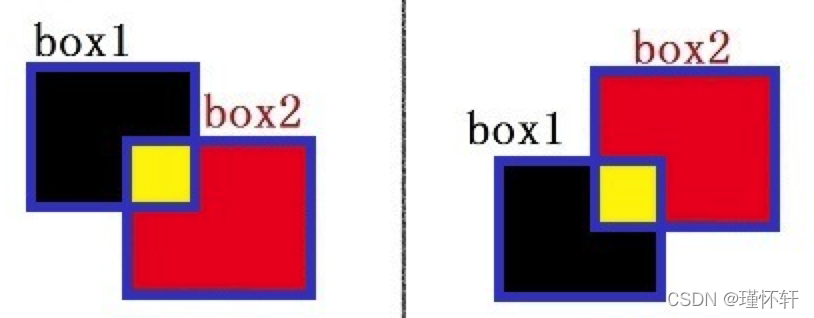
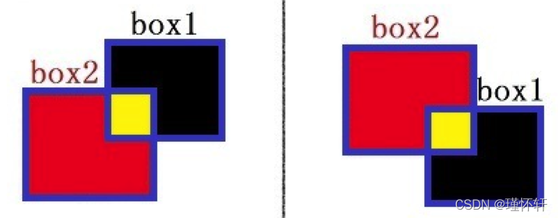
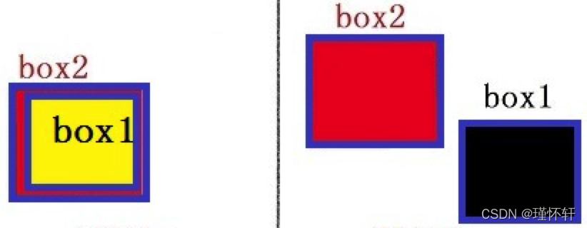
起初这样考虑没有一点问题，也能实现想要的效果。那抛给你一个问题先思考下，如何将这几种清晰合并？这也是1--->N--->1 的过程。

我们重新思考一下，两个交集的计算，现在我们先降维思考一下一维如何求交集。

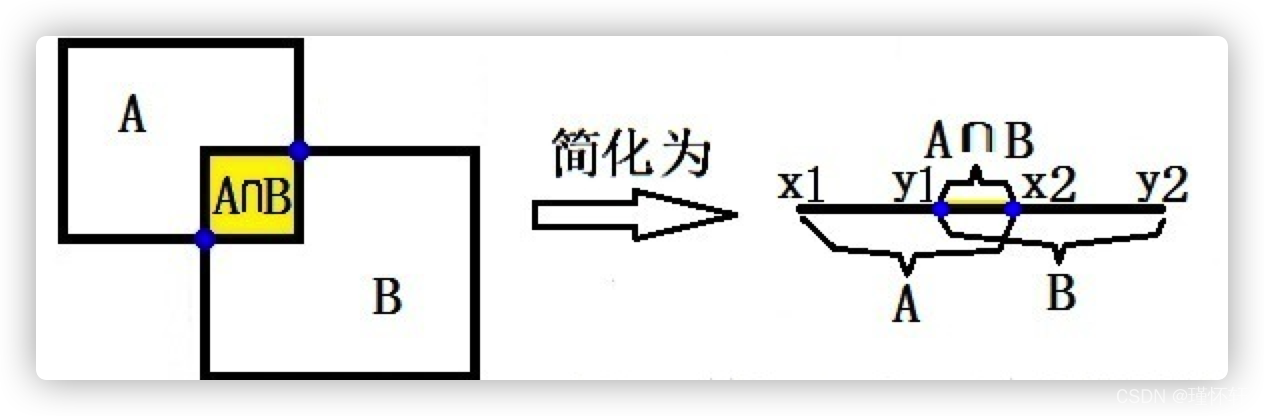
可能看不懂这个图，你可以想象一下，我将左侧图上下一拍，压成了右图，变成一个一维的。

这样我们计算一维交集的关键是找交集左右边界，有就是右图中的蓝点。

现在先忘记我们左侧要干的事情，先看右侧。假设集合A[x1,x2],集合B[y1,y2] 然后AB交集的上下界限的计算逻辑如下：

交集下界 z1 ：x1和y1的最大值为下界。公式表示为： max(x1,y1)
交集上界 z2 : x2 和与y2最小值为上界。公式表示为 : min(x2,y2)
如果 z2 - z1 小于0，则表示没有交集，（就相当于x2 - y1 < 0 , 说明y1 > x2 ,y1在 x2 右侧所以不能相交。）

下面使用python实现两个一维集合的IoU的计算：

def iou(set_a, set_b):
    '''
    一维 iou 的计算
    '''
    x1, x2 = min(set_a) , max(set_a) # (left, right)      取出集合的左右两界
    y1, y2 = min(set_b) , max(set_b) # (left, right)
    
    low = max(x1, y1)        #根据公式计算 交集 上下界
    high = min(x2, y2)

    # intersection        #分情况判断 计算交集
    if high-low<0:        #不相交
        inter = 0
    else:
        inter = high-low   
    # union               #求并集
    union = (x2 - x1) + (y2 - y1) - inter
    # iou
    iou = inter / union   #计算一维的IoU
    return iou

计算了两个一维集合的 iou，将上面的程序进行扩展，即可得到二维IoU 计算的程序。

本质就是把👆🏻图中左侧部分取出来。刚才不是上下方向拍了一次变成一维。其实就是计算的二维中w方向的交集。现在我们从左右两侧进行拍一次，从而计算h方向的交集。

def iou(box1, box2):
    '''
    两个框（二维）的 iou 计算
    
    注意：边框以左上为原点
    
    box:[top, left, bottom, right]       #bounding box的 左上和右下坐标
    '''
    # 在h方向压一次，并计算 交集，这里程序简化了
    in_h = min(box1[2], box2[2]) - max(box1[0], box2[0]) 
    # 在w方向压一次
    in_w = min(box1[3], box2[3]) - max(box1[1], box2[1])
    #分别从两个方向进行判断，两个框是否不相交。任意一个方向不相交，那么两个框都不会相交。
    inter = 0 if in_h<0 or in_w<0 else in_h*in_w
    
    #交集求来，并集很好算了。
    union = (box1[2] - box1[0]) * (box1[3] - box1[1]) + \
            (box2[2] - box2[0]) * (box2[3] - box2[1]) - inter
    iou = inter / union
    return iou

再往深入思考一下，三维也是一个道理，在z方向再拍一次。分别计算就可以了。就可以判断目标在三维坐标系中是否碰撞，重合。这里就不演示了，有时间可以自己推理了。

TensorFlow上实现IoU：

import tensorflow as tf

def IoU_calculator(x, y, w, h, l_x, l_y, l_w, l_h):
    """calaulate IoU
    Args:
    预测框
      x: net predicted x
      y: net predicted y
      w: net predicted width
      h: net predicted height
    真实框
      l_x: label x
      l_y: label y
      l_w: label width
      l_h: label height
    
    Returns:
      IoU
    """
    
    # convert to coner  
    #原先坐标【left,top,width,height】 --> 【left,top,right,bottom】
    x_max = x + w/2
    y_max = y + h/2
    x_min = x - w/2
    y_min = y - h/2
 
    l_x_max = l_x + l_w/2
    l_y_max = l_y + l_h/2
    l_x_min = l_x - l_w/2
    l_y_min = l_y - l_h/2

    # calculate the inter
    #使用tf.minimum 计算最小值 
    #在x方向拍
    inter_x_max = tf.minimum(x_max, l_x_max)
    inter_x_min = tf.maximum(x_min, l_x_min)
    #在y方向拍
    inter_y_max = tf.minimum(y_max, l_y_max)
    inter_y_min = tf.maximum(y_min, l_y_min)
    #计算交集
    inter_w = inter_x_max - inter_x_min
    inter_h = inter_y_max - inter_y_min
    #判断
    inter = tf.cond(tf.logical_or(tf.less_equal(inter_w,0), tf.less_equal(inter_h,0)), 
                    lambda:tf.cast(0,tf.float32), 
                    lambda:tf.multiply(inter_w,inter_h))
    # calculate the union，计算并集
    union = w*h + l_w*l_h - inter
    
    IoU = inter / union
    return IoU

在模型网络中的实现

# -*- coding: utf-8 -*-
#
# This is the python code for calculating bbox IoU,
# By running the script, we can get the IoU score between pred / gt bboxes
#
# Author: hzhumeng01 2018-10-19
# copyright @ netease, AI group

from __future__ import print_function, absolute_import
import numpy as np

def get_IoU(pred_bbox, gt_bbox):
    """
    return iou score between pred / gt bboxes
    :param pred_bbox: predict bbox coordinate
    :param gt_bbox: ground truth bbox coordinate
    :return: iou score
    """

    # bbox should be valid, actually we should add more judgements, just ignore here...
    # assert ((abs(pred_bbox[2] - pred_bbox[0]) > 0) and
    #         (abs(pred_bbox[3] - pred_bbox[1]) > 0))
    # assert ((abs(gt_bbox[2] - gt_bbox[0]) > 0) and
    #         (abs(gt_bbox[3] - gt_bbox[1]) > 0))

    # -----0---- get coordinates of inters
    ixmin = max(pred_bbox[0], gt_bbox[0])
    iymin = max(pred_bbox[1], gt_bbox[1])
    ixmax = min(pred_bbox[2], gt_bbox[2])
    iymax = min(pred_bbox[3], gt_bbox[3])
    iw = np.maximum(ixmax - ixmin + 1., 0.)
    ih = np.maximum(iymax - iymin + 1., 0.)

    # -----1----- intersection
    inters = iw * ih

    # -----2----- union, uni = S1 + S2 - inters
    uni = ((pred_bbox[2] - pred_bbox[0] + 1.) * (pred_bbox[3] - pred_bbox[1] + 1.) +
           (gt_bbox[2] - gt_bbox[0] + 1.) * (gt_bbox[3] - gt_bbox[1] + 1.) -
           inters)

    # -----3----- iou
    overlaps = inters / uni

    return overlaps


def get_max_IoU(pred_bboxes, gt_bbox):
    """
    given 1 gt bbox, >1 pred bboxes, return max iou score for the given gt bbox and pred_bboxes
    :param pred_bbox: predict bboxes coordinates, we need to find the max iou score with gt bbox for these pred bboxes
    :param gt_bbox: ground truth bbox coordinate
    :return: max iou score
    """

    # bbox should be valid, actually we should add more judgements, just ignore here...
    # assert ((abs(gt_bbox[2] - gt_bbox[0]) > 0) and
    #         (abs(gt_bbox[3] - gt_bbox[1]) > 0))

    if pred_bboxes.shape[0] > 0:
        # -----0---- get coordinates of inters, but with multiple predict bboxes
        ixmin = np.maximum(pred_bboxes[:, 0], gt_bbox[0])
        iymin = np.maximum(pred_bboxes[:, 1], gt_bbox[1])
        ixmax = np.minimum(pred_bboxes[:, 2], gt_bbox[2])
        iymax = np.minimum(pred_bboxes[:, 3], gt_bbox[3])
        iw = np.maximum(ixmax - ixmin + 1., 0.)
        ih = np.maximum(iymax - iymin + 1., 0.)

        # -----1----- intersection
        inters = iw * ih

        # -----2----- union, uni = S1 + S2 - inters
        uni = ((gt_bbox[2] - gt_bbox[0] + 1.) * (gt_bbox[3] - gt_bbox[1] + 1.) +
               (pred_bboxes[:, 2] - pred_bboxes[:, 0] + 1.) * (pred_bboxes[:, 3] - pred_bboxes[:, 1] + 1.) -
               inters)

        # -----3----- iou, get max score and max iou index
        overlaps = inters / uni
        ovmax = np.max(overlaps)
        jmax = np.argmax(overlaps)

    return overlaps, ovmax, jmax

if __name__ == "__main__":

    # test1
    pred_bbox = np.array([50, 50, 90, 100])   # top-left: <50, 50>, bottom-down: <90, 100>, <x-axis, y-axis>
    gt_bbox = np.array([70, 80, 120, 150])
    print (get_IoU(pred_bbox, gt_bbox))
    
    # test2
    pred_bboxes = np.array([[15, 18, 47, 60],
                          [50, 50, 90, 100],
                          [70, 80, 120, 145],
                          [130, 160, 250, 280],
                          [25.6, 66.1, 113.3, 147.8]])
    gt_bbox = np.array([70, 80, 120, 150])
    print (get_max_IoU(pred_bboxes, gt_bbox))

其中：1、其中加1，应该是给边界重合给点冗余。2、下面获取最大IoU 函数是在去重的时候使用。

关键代码：

ixmin = max(pred_bbox[0], gt_bbox[0])
iymin = max(pred_bbox[1], gt_bbox[1])
ixmax = min(pred_bbox[2], gt_bbox[2])
iymax = min(pred_bbox[3], gt_bbox[3])
iw = np.maximum(ixmax - ixmin + 1., 0.)
ih = np.maximum(iymax - iymin + 1., 0.)

1.1、如何计算 mIoU？

知道这是干嘛的就行，实现可能在研究分割时再掌握。

Mean Intersection over Union(MIoU，均交并比)，为语义分割的标准度量。其计算两个集合的交集和并集之比，在语义分割问题中，这两个集合为真实值（ground truth）和预测值（predicted segmentation）。这个比例可以变形为TP（交集）比上TP、FP、FN之和（并集）。在每个类上计算IoU，然后取平均。 pij表示真实值为i，被预测为j的数量。

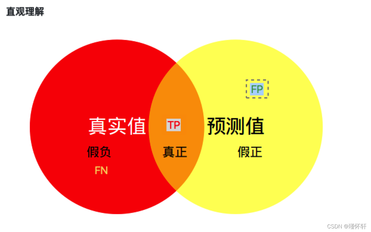
$MIoU=\frac{1}{k+1}\sum^{k}{i=0}{\frac{p{ii}}{\sum_{j=0}^{k}{p_{ij}+\sum_{j=0}^{k}{p_{ji}-p_{ii}}}}}$

红色圆代表真实值，黄色圆代表预测值。橙色部分为两圆交集部分。

MPA（Mean Pixel Accuracy，均像素精度）：计算橙色与红色圆的比例；
MIoU：计算两圆交集（橙色部分）与两圆并集（红色+橙色+黄色）之间的比例，理想情况下两圆重合，比例为1。

下图代码解析参考博客

import numpy as np
import argparse
import json
from PIL import Image
from os.path import join

#设标签宽W，长H
def fast_hist(a, b, n):#a是转化成一维数组的标签，形状(H×W,)；b是转化成一维数组的标签，形状(H×W,)；n是类别数目，实数（在这里为19）
    '''
	核心代码
	'''
    k = (a >= 0) & (a < n)#k是一个一维bool数组，形状(H×W,)；目的是找出标签中需要计算的类别（去掉了背景）
    return np.bincount(n * a[k].astype(int) + b[k], minlength=n ** 2).reshape(n, n)#np.bincount计算了从0到n**2-1这n**2个数中每个数出现的次数，返回值形状(n, n)


def per_class_iu(hist):#分别为每个类别（在这里是19类）计算mIoU，hist的形状(n, n)
    '''
	核心代码
	'''
    return np.diag(hist) / (hist.sum(1) + hist.sum(0) - np.diag(hist))#矩阵的对角线上的值组成的一维数组/矩阵的所有元素之和，返回值形状(n,)


def label_mapping(input, mapping):#主要是因为CityScapes标签里面原类别太多，这样做把其他类别转换成算法需要的类别（共19类）和背景（标注为255）
    output = np.copy(input)#先复制一下输入图像
    for ind in range(len(mapping)):
        output[input == mapping[ind][0]] = mapping[ind][1]#进行类别映射，最终得到的标签里面之后0-18这19个数加255（背景）
    return np.array(output, dtype=np.int64)#返回映射的标签
'''
compute_mIoU函数是以CityScapes图像分割验证集为例来计算mIoU值的
由于作者个人贡献的原因，本函数除了最主要的计算mIoU的代码之外，还完成了一些其他操作，
比如进行数据读取，因为原文是做图像分割迁移方面的工作，因此还进行了标签映射的相关工作，在这里笔者都进行注释。
大家在使用的时候，可以忽略原作者的数据读取过程，只需要注意计算mIoU的时候每张图片分割结果与标签要配对。
主要留意mIoU指标的计算核心代码即可。
'''
def compute_mIoU(gt_dir, pred_dir, devkit_dir=''):#计算mIoU的函数
    """
    Compute IoU given the predicted colorized images and 
    """
    with open(join(devkit_dir, 'info.json'), 'r') as fp: #读取info.json，里面记录了类别数目，类别名称，标签映射方式等等。
      info = json.load(fp)
    num_classes = np.int(info['classes'])#读取类别数目，这里是19类，详见博客中附加的info.json文件
    print('Num classes', num_classes)#打印一下类别数目
    name_classes = np.array(info['label'], dtype=np.str)#读取类别名称，详见博客中附加的info.json文件
    mapping = np.array(info['label2train'], dtype=np.int)#读取标签映射方式，详见博客中附加的info.json文件
    hist = np.zeros((num_classes, num_classes))#hist初始化为全零，在这里的hist的形状是[19, 19]

    image_path_list = join(devkit_dir, 'val.txt')#在这里打开记录验证集图片名称的txt
    label_path_list = join(devkit_dir, 'label.txt')#在这里打开记录验证集标签名称的txt
    gt_imgs = open(label_path_list, 'r').read().splitlines()#获得验证集标签名称列表
    gt_imgs = [join(gt_dir, x) for x in gt_imgs]#获得验证集标签路径列表，方便直接读取
    pred_imgs = open(image_path_list, 'r').read().splitlines()#获得验证集图像分割结果名称列表
    pred_imgs = [join(pred_dir, x.split('/')[-1]) for x in pred_imgs]#获得验证集图像分割结果路径列表，方便直接读取

    for ind in range(len(gt_imgs)):#读取每一个（图片-标签）对
        pred = np.array(Image.open(pred_imgs[ind]))#读取一张图像分割结果，转化成numpy数组
        label = np.array(Image.open(gt_imgs[ind]))#读取一张对应的标签，转化成numpy数组
        label = label_mapping(label, mapping)#进行标签映射（因为没有用到全部类别，因此舍弃某些类别），可忽略
        if len(label.flatten()) != len(pred.flatten()):#如果图像分割结果与标签的大小不一样，这张图片就不计算
            print('Skipping: len(gt) = {:d}, len(pred) = {:d}, {:s}, {:s}'.format(len(label.flatten()), len(pred.flatten()), gt_imgs[ind], pred_imgs[ind]))
            continue
        hist += fast_hist(label.flatten(), pred.flatten(), num_classes)#对一张图片计算19×19的hist矩阵，并累加
        if ind > 0 and ind % 10 == 0:#每计算10张就输出一下目前已计算的图片中所有类别平均的mIoU值
            print('{:d} / {:d}: {:0.2f}'.format(ind, len(gt_imgs), 100*np.mean(per_class_iu(hist))))
    
    mIoUs = per_class_iu(hist)#计算所有验证集图片的逐类别mIoU值
    for ind_class in range(num_classes):#逐类别输出一下mIoU值
        print('===>' + name_classes[ind_class] + ':\t' + str(round(mIoUs[ind_class] * 100, 2)))
    print('===> mIoU: ' + str(round(np.nanmean(mIoUs) * 100, 2)))#在所有验证集图像上求所有类别平均的mIoU值，计算时忽略NaN值
    return mIoUs


def main(args):
   compute_mIoU(args.gt_dir, args.pred_dir, args.devkit_dir)#执行计算mIoU的函数


if __name__ == "__main__":
    parser = argparse.ArgumentParser()
    parser.add_argument('gt_dir', type=str, help='directory which stores CityScapes val gt images')#设置gt_dir参数，存放验证集分割标签的文件夹
    parser.add_argument('pred_dir', type=str, help='directory which stores CityScapes val pred images')#设置pred_dir参数，存放验证集分割结果的文件夹
    parser.add_argument('--devkit_dir', default='dataset/cityscapes_list', help='base directory of cityscapes')#设置devikit_dir文件夹，里面有记录图片与标签名称及其他信息的txt文件
    args = parser.parse_args()
    main(args)#执行主函数

Pytorch 计算 MIoU 源码：

基本思路就是把只保留一类的IoU，其他类IoU置零，然后最后将mIoU * num_classes就可以了。

class IOUMetric:
    """
    Class to calculate mean-iou using fast_hist method
    """

    def __init__(self, num_classes):
        self.num_classes = num_classes
        self.hist = np.zeros((num_classes, num_classes))

    def _fast_hist(self, label_pred, label_true):
        mask = (label_true >= 0) & (label_true < self.num_classes)
        hist = np.bincount(
            self.num_classes * label_true[mask].astype(int) +
            label_pred[mask], minlength=self.num_classes ** 2).reshape(self.num_classes, self.num_classes)
        return hist

    def add_batch(self, predictions, gts):
        for lp, lt in zip(predictions, gts):
            self.hist += self._fast_hist(lp.flatten(), lt.flatten())

    def evaluate(self):
        acc = np.diag(self.hist).sum() / self.hist.sum()
        acc_cls = np.diag(self.hist) / self.hist.sum(axis=1)
        acc_cls = np.nanmean(acc_cls)
        iu = np.diag(self.hist) / (self.hist.sum(axis=1) + self.hist.sum(axis=0) - np.diag(self.hist))
        mean_iu = np.nanmean(iu)
        freq = self.hist.sum(axis=1) / self.hist.sum()
        fwavacc = (freq[freq > 0] * iu[freq > 0]).sum()
        return acc, acc_cls, iu, mean_iu, fwavacc

Python 简单版本实现：

#RT:RightTop
#LB:LeftBottom
def IOU(rectangle A, rectangleB):
    W = min(A.RT.x, B.RT.x) - max(A.LB.x, B.LB.x)
    H = min(A.RT.y, B.RT.y) - max(A.LB.y, B.LB.y)
    if W <= 0 or H <= 0:
        return 0;
    SA = (A.RT.x - A.LB.x) * (A.RT.y - A.LB.y)
    SB = (B.RT.x - B.LB.x) * (B.RT.y - B.LB.y)
    cross = W * H
    return cross/(SA + SB - cross)

1.2、IoU变体

目标检测基础模块之IoU及优化 - 知乎1 简介 IoU又名交并比，是一种计算不同图像相互重叠比例的算法，时常被用于深度学习领域的目标检测或语义分割任务中。 1.1 IoU在目标检测中的应用在目标检测任务中，我们时常会让模型一次性生成大量的候选框（can…https://zhuanlan.zhihu.com/p/111013447

二、mAP

mAP定义和相关概念，还是下图拿来看，容易理解：不要和IoU中的图混淆。

mAP：mean Average Precision, 各类AP的平均值。【mean Average Precision】
AP：A由Recall和Precision两个维度下曲线下面包围的面积【Average Precision】
PR曲线：Precision-Recall曲线
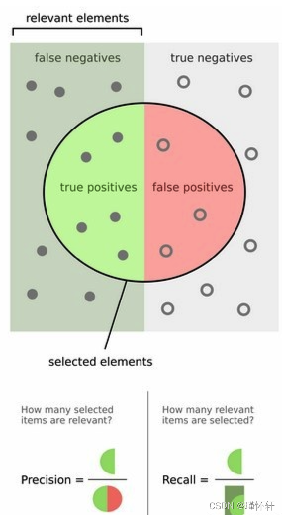
Precision：TP/(TP+FP) 【注】预测对的真实样本 / 所有预测样本；橘 / 橘+黄
Recall：TP / (TP + FN) 【注】预测对的正样本 / 所有真实样本；橘色 / 橘＋红
TP : 在判定为positive的样本中，判断正确的数目。【Ture Positive】
FP：在判定为positive的样本中，判断错误的数目。【False Positive】
TN ：在判定为negative的样本中，判断正确的数目。【True Negative】
FN ：在判定为negative的样本中，判断错误的数目。【False Negative】

有时论文中出现Iou阈值，是在阈值筛选后计算以上各值。

总结：

AP衡量的是模型在每个类别上的好坏，mAP衡量的是模型在所有类别上的好坏，得到AP后mAP的计算就变得很简单了，就是取所有类别AP的平均值。

代码分析：

# VOC-style mAP，分为两个计算方式，之所有两个计算方式，是因为2010年后VOC更新了评估方法，因此就有了07-metric和else...
def voc_ap(rec, prec, use_07_metric=False):
    """
    average precision calculations
    [precision integrated to recall]
    :param rec: recall list
    :param prec: precision list
    :param use_07_metric: 2007 metric is 11-recall-point based AP
    :return: average precision
    """
    if use_07_metric:
        # 11 point metric
        ap = 0.
        # VOC07是11点插值的AP方式，等于是卡了11个离散的点，划分10个区间来计算AP
        for t in np.arange(0., 1.1, 0.1):
            if np.sum(rec >= t) == 0:
                p = 0    # recall卡的阈值到顶了，1.1
            else:
                p = np.max(prec[rec >= t])   # VOC07：选择每个recall区间内对应的最高precision的计算方案
            ap = ap + p / 11.    # 11-recall-point based AP
    else:
        # correct AP calculation
        # first append sentinel values at the end
        mrec = np.concatenate(([0.], rec, [1.]))
        mpre = np.concatenate(([0.], prec, [0.]))

        # compute the precision envelope
        for i in range(mpre.size - 1, 0, -1):
            mpre[i - 1] = np.maximum(mpre[i - 1], mpre[i])    # 这个是不是动态规划？从后往前找之前区间内的top-precision，多么优雅的代码呀~~~

        # to calculate area under PR curve, look for points where X axis (recall) changes value
        # 上面的英文，可以结合着fig 2的绿框理解，一目了然
        # VOC10是是根据recall值变化的区间来计算的，如果recall变化很多次，就可以认为是一种 “伪” 连续的方式计算了，以下求的是recall的变化
        i = np.where(mrec[1:] != mrec[:-1])[0]

        # 计算AP，这个计算方式有点玄乎，是一个积分公式的简化，应该是对应的fig 2中红色曲线以下的面积，之前公式的推导我有看过，现在有点忘了，麻烦各位同学补充一下
        # 现在理解了，不难，公式：sum (\Delta recall) * prec，其实结合fig2和下面的图，不就是算的积分么？如果recall划分得足够细，就可以当做连续数据，然后以下公式就是积分公式，算的precision、recall下面的面积了
        ap = np.sum((mrec[i + 1] - mrec[i]) * mpre[i + 1])
    return ap

通常VOC10标准下计算的mAP值会高于VOC07，原因如下

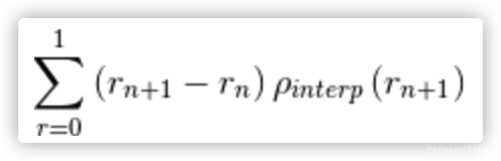
插值平均精度：通常称其为平均精度。使用 P(k)代替，在 k 个图像的检索截止处的精度，插值平均精度使用一下公式：

换句话说，插值平均精度不是使用在截止 k 处实际观察到的精度，而是使用在所有具有更高召回率的截止上观察到的最大精度。计算插值平均精度的完整方程为：

从视觉上看，这是插值平均精度与近似平均精度的比较（为了显示更有趣的图，这不是来自前面的示例）

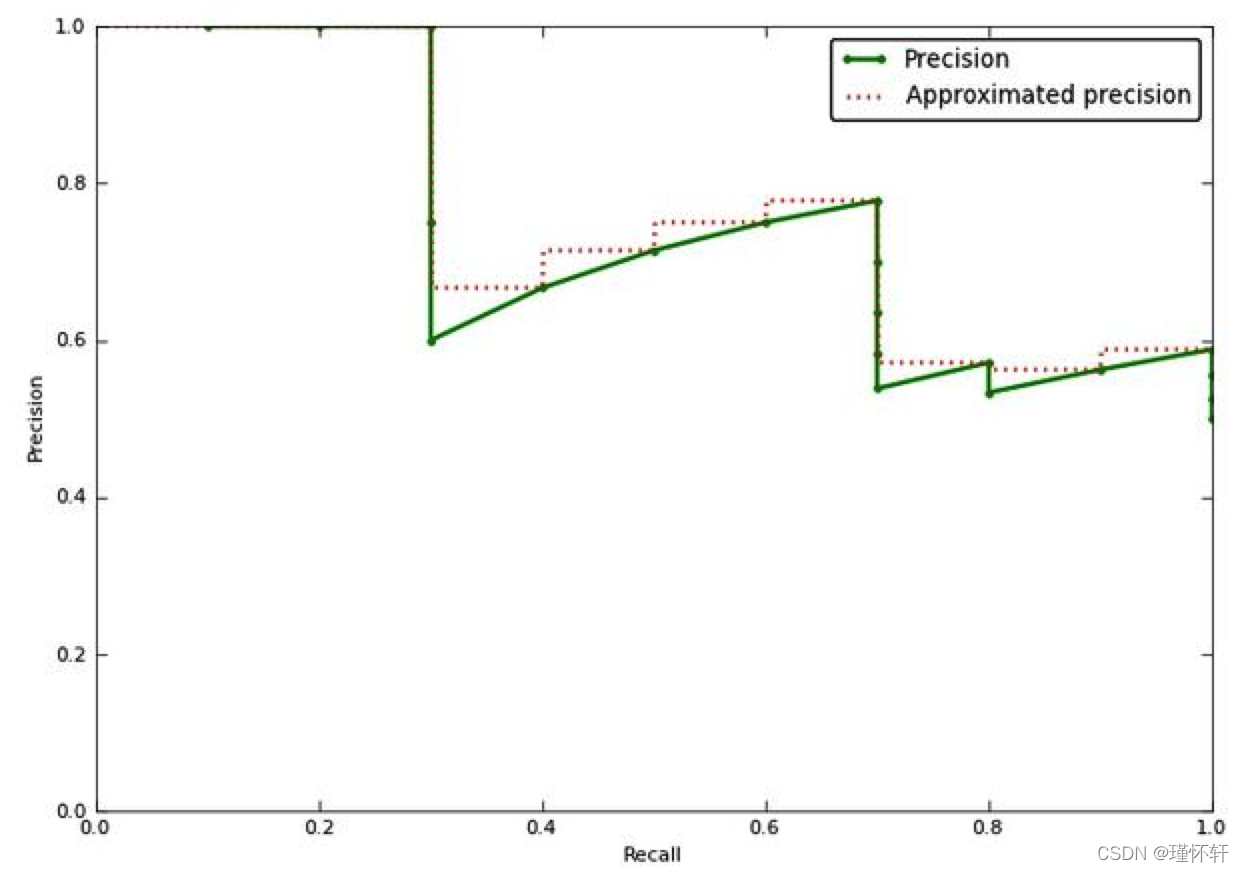
近似的平均精度与实际观察到的曲线非常接近。插值平均精度高估了许多点的精度，并产生比近似平均精度更高的平均精度值。

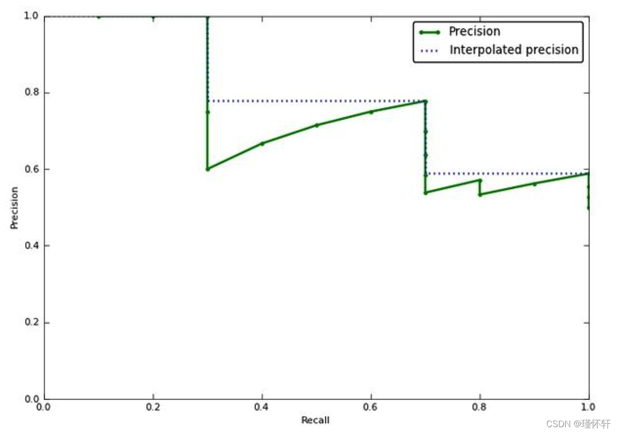
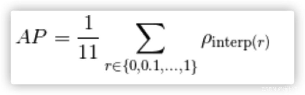
在VOC2010以前，只需要选取当Recall >= 0, 0.1, 0.2, ..., 1共11个点时的Precision最大值，然后AP就是这11个Precision的平均值。在VOC2010及以后，需要针对每一个不同的Recall值（包括0和1），选取其大于等于这些Recall值时的Precision最大值，然后计算PR曲线下面积作为AP值。

1）11-point interpolation（VOC07，10之前）

11-point interpolation通过平均一组11个等间距的Recall值[0,0.1,0.2，...，1]对应的Precision来绘制P-R曲线.

计算precision时采用一种插值方法（interpolate），即对于某个recall值r，precision值取所有recall>=r中的最大值（这样保证了p-r曲线是单调递减的，避免曲线出现抖动）

2）Interpolating all points（VOC10之后）

详细研究参考：

Detection基础模块之（二）mAP_一个新新的小白的博客-CSDN博客

机器学习--PR曲线， ROC曲线 - 老张哈哈哈 - 博客园

【目标检测】VOC mAP - 知乎

2.1 PR 曲线

PR曲线用途：当confidence阈值改变时，衡量模型的performance

好模型的标志：PR曲线鼓大（靠近右上方）,见下图示例，recall变大时precision下降小，意味着模型不需要通过预测更多的BBOX来检测出GT。对于好的模型，当confidence阈值改变，precision和recall都保持在较高水平

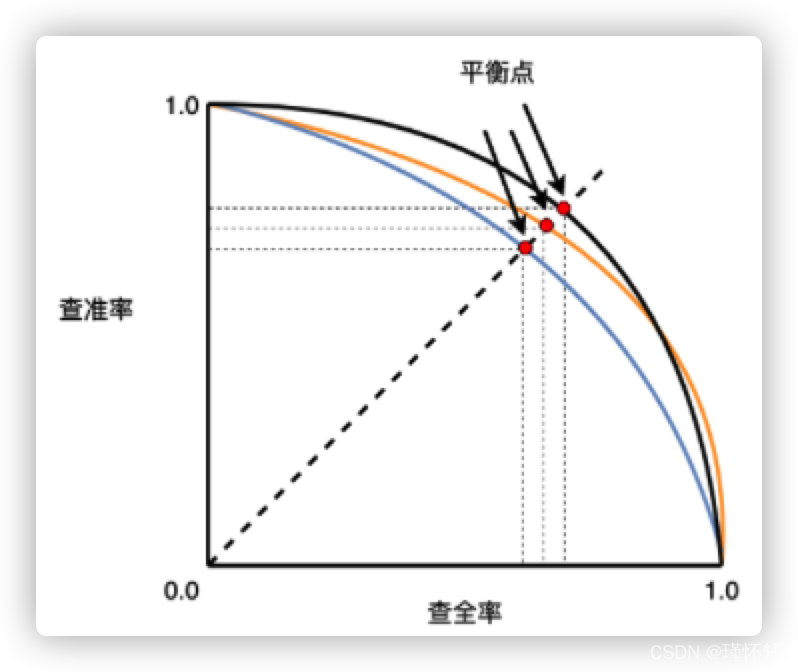
AP：PR曲线下面积的近似，是一个0~1之间的数值，也可用来衡量模型的performance

AP VS PR曲线：

PR曲线比较直观，但由于曲线的上下震荡，不方便比较不同模型的PR曲线
AP是一个数字，模型的AP大，则模型更好，方便比较不同模型

2.2、速度指标

1）FPS，检测器每秒能处理图片的张数。

2）检测器处理每张图片所需要的时间。

但速度评价指标必须在同一硬件上进行，同一硬件，它的最大FLOPS（每秒运算浮点数代表着硬件性能，此处区分FLOPs）是相同的，不同网络，处理每张图片所需的FLOPs(浮点操作数)是不同的，所以同一硬件处理相同图片所需的FLOPs越小，相同时间内，就能处理更多的图片，速度也就越快，处理每张图片所需的FLOPs与许多因素有关，比如你的网络层数，参数量，选用的激活函数等等，这里仅谈一下网络的参数量对其的影响，一般来说参数量越低的网络，FLOPs会越小，保存模型所需的内存小，对硬件内存要求比较低，因此比较对嵌入式端较友好。

2.2.1、FLOPs和FLOPS区分

FLOPs：floating point operations 指的是浮点运算次数，理解为计算量，可以用来衡量算法/模型的复杂度。此处区分一下FLOPS（全部大写），FLOPS指的是每秒运算的浮点数，理解为计算速度，衡量一个硬件的标准。我们要的是衡量模型的复杂度的指标，所以选择FLOPs。

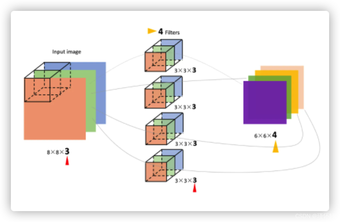
（1）卷积层

FLOPs计算（以下计算FLOPs不考虑激活函数的运算）

FLOPs=(2*Ci*k*K-1）*H*W*Co（不考虑bias）

FLOPs=(2*Ci*k*K）*H*W*Co（考虑bias）

Ci为输入特征图通道数，K为过滤器尺寸，H,W,Co为输出特征图的高，宽和通道数。

左边是乘法运算量，右边是加法运算量,因为n个数字要加n-1次，所以有个-1.这里忽略了bais如果算上bais需要把-1去掉。

公式中2是因为一个MAC算2个 operations，不考虑bias时有-1，有bias时没有-1。

MAC：乘积累加运算，是在数字信号处理器或一些微处理器中的特殊运算。许多运算（例如卷积运算、点积运算、矩阵运算、数字滤波器运算、乃至多项式的求值运算）都可以分解为数个 MAC 指令，可以提高运算效率

（2）池化层

池化分为最大值池化和均值池化，网络中一般池化层较少，且池化操作所占用的FLOPs很少，对速度性能影响较小。

最大池化一般是找出输入特征图中过滤器范围内的最大值，以最大值代替，好像不涉及到浮点运算操作。

设输入图像尺寸为W * W * 3，卷积核尺寸为F，步幅为S（池化时，例如最大池化或平均池化，S的大小通常小于等于F，使每个区域没有重叠），池化一般化不用padding，也没有类似于卷积核个数的概念(所以经过pooling后，一般化channel不变，变的只是每个channel的大小)，则经过该池化层后输出的图像尺寸为：

[(W-F)/S + 1 ] * [(W-F)/S + 1] * 3

注：池化层参数存在计算(平均池化，最大池化) ，它就在卷积区域求最大值和平均值，基本可以忽略。

（3) 全连接层

CNN基本用FCN来代表，可用卷积层来实现全连接层的功能。设I为输入神经元个数，O为输出神经元个数，输出的每个神经元都是由输入的每个神经元乘以权重（浮点操作数为I），然后把所得的积的和相加（浮点操作数为I-1），加上一个偏差（浮点操作数为1）得到了，故FLOPs为：

FLOPs=(I+I-1) * O = (2I-1) * O(不考虑bias)

FLOPs=((I+I-1+1）* O = (2I) * O(考虑bias)

计算FLOPs小工具：

https://github.com/swimmant/pytorch-OpCounterhttps://github.com/swimmant/pytorch-OpCounter

三、候选区域（region proposal）

候选区域（region proposal）：在目标检测初期使用的是窗口滑动的思想后来通常使用算法先来预测一下要检测的目标在极可能出现在图像的哪块区域，通常采用selective search的方法，（region proposal在R-CNN 论文中有提到这块内容）

selective search的方法：（白话）对图像中的每个像素进行聚类（相邻的相同颜色的像素是一个类别，相邻的相同纹理像素是一个类别。这样就让图像变成下图，类似k-近邻分类算法的分类效果图）多块斑状图，每一个斑都很可能是我们需要检测的目标。

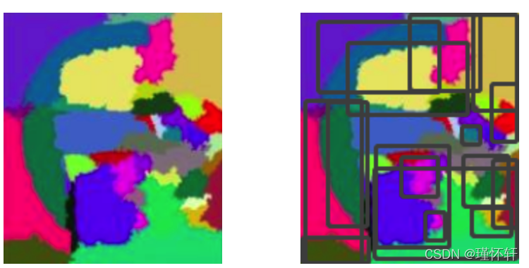
生成的块状斑，具有低耦合高内聚的特点。每一块之间的差异较大，块内的像素点和像素点之间差异小。

斑的正外接矩形便是产生的region propoal。

一张图可能很产生很多个proposal，筛选候选区域（region proposal）使用IoU阈值的方式进行减少低可能性的proposal。

R-CNN 中的region proposals 起的作用: 为后续的CNN网络提供输入。这里不展开讲了~~

四、非极大抑制（NMS）

非极大抑制（NMS）：当图像中预测多个预测框（Bounding box，bbox）时，预测框之间可能存在高冗余（一个目标预测了多个矩形框），需要过滤一些相似的结果。简而言之，NMS用于剔除图像中预测的冗余bbox。

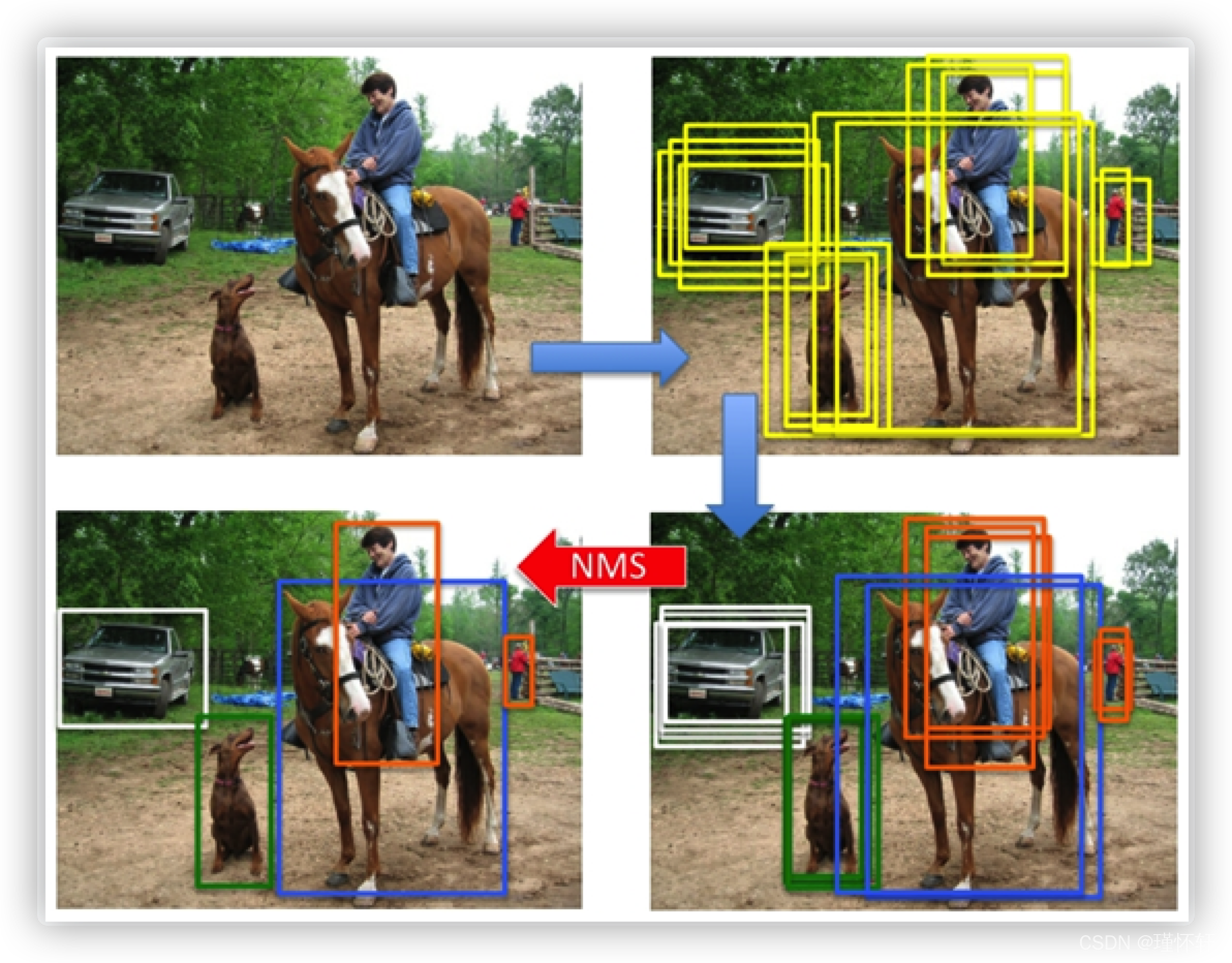
每个类分别进行NMS，不同的类的score无影响，相同的类的score会有影响。

单类NMS算法思想：

1、对该类（🍊类）所有的预测框（Bbox）的分数（置信度、score）进行降序排序，得到排序集合B{ }

2、选择score最高的那个检测框M，将它从排序集B{ }中删除加入结果集D{ }

3、分别计算集合B{ }中的Bbox与得分最高检测框M的IoU，如果高于一个阈值T，认为他们是同一个物体，将他们从集合B{ }中删除，如果低于某个阈值T，认为同类的不同物体，保留下来。

4、调转到步骤2，直到B { } 为空。

5、输入结果集合D { },得到去除冗余框的 Bbox集合

【注】上一步，筛选完后属于第一个该类（🍊类）的目标的Bbox确定在结果集D{ }；如果集合B{ }还有剩余该类，说明该类还有第二个目标，再选一个最高分，再计算剩余的和它的iou并删除，循环往复，直至B中没有剩余的Bbox。（这一步算法上来说是相同操作，直接放入循环中就行了，此处只是解释）

多类NMS算法，再类别层面进行循环。

单类别NMS实现：

def py_cpu_nms(dets, thresh):
    """Pure Python NMS baseline."""
    #x1、y1、x2、y2、以及score赋值
    x1 = dets[:, 0]
    y1 = dets[:, 1]
    x2 = dets[:, 2]
    y2 = dets[:, 3]
    scores = dets[:, 4]

    #每一个检测框的面积
    areas = (x2 - x1 + 1) * (y2 - y1 + 1)
    #按照score置信度降序排序
    order = scores.argsort()[::-1]

    keep = [] #保留的结果框集合
    while order.size > 0:
        i = order[0]
        keep.append(i) #保留该类剩余box中得分最高的一个
        #得到相交区域,左上及右下
        xx1 = np.maximum(x1[i], x1[order[1:]])
        yy1 = np.maximum(y1[i], y1[order[1:]])
        xx2 = np.minimum(x2[i], x2[order[1:]])
        yy2 = np.minimum(y2[i], y2[order[1:]])

        #计算相交的面积,不重叠时面积为0
        w = np.maximum(0.0, xx2 - xx1 + 1)
        h = np.maximum(0.0, yy2 - yy1 + 1)
        inter = w * h
        #计算IoU：重叠面积 /（面积1+面积2-重叠面积）
        ovr = inter / (areas[i] + areas[order[1:]] - inter)
        #保留IoU小于阈值的box
        inds = np.where(ovr <= thresh)[0]
        order = order[inds + 1] #因为ovr数组的长度比order数组少一个,所以这里要将所有下标后移一位
       
    return keep

RBF网络中NMS实现：

out = net(x)      # forward pass，这里相当于将图像 x 输入RFBNet，得到了pred cls + reg
boxes, scores = detector.forward(out,priors) # 结合priors，将pred reg（也即预测的offsets）解码成最终的pred bbox，如果理解anchor / default bbox操作流程，这个应该很好理解的；
boxes = boxes[0]
scores=scores[0]

# scale each detection back up to the image
boxes *= scale   # （0，1）区间坐标的bbox做尺度反正则化
boxes = boxes.cpu().numpy()
scores = scores.cpu().numpy()

for j in range(1, num_classes):      # 对每个类 j 的pred bbox单独做NMS，为什么index从1开始？因为0是bg，做NMS无意义
    inds = np.where(scores[:, j] > thresh)[0]     # 找到该类 j 下，所有cls score大于thresh的bbox，为什么选择大于thresh的bbox？因为score小于阈值的bbox，直接可以过滤掉，无需劳烦NMS
    if len(inds) == 0:    # 没有满足条件的bbox，返回空，跳过；
        all_boxes[j][i] = np.empty([0, 5], dtype=np.float32)
        continue
    c_bboxes = boxes[inds]
    c_scores = scores[inds, j]   # 找到对应类 j 下的score即可
    c_dets = np.hstack((c_bboxes, c_scores[:, np.newaxis])).astype(
        np.float32, copy=False)   # 将满足条件的bbox + cls score的bbox通过hstack完成合体

    keep = nms(c_dets, 0.45, force_cpu=args.cpu)    # NMS，返回需保存的bbox index：keep
    c_dets = c_dets[keep, :]
    all_boxes[j][i] = c_dets     # i 对应每张图像，j 对应图像中类别 j 的bbox清单

【注】for j in range(1, num_classes)操作表明了，NMS是逐类进行的，也即参与NMS的bbox都属于同一类；

pytorch实现代码：

# Original author: Francisco Massa:
# https://github.com/fmassa/object-detection.torch
# Ported to PyTorch by Max deGroot (02/01/2017)
def nms(boxes, scores, overlap=0.5, top_k=200):
    """Apply non-maximum suppression at test time to avoid detecting too many
    overlapping bounding boxes for a given object. ---- 这里面有一个细节，NMS仅用于测试阶段，为什么不用于训练阶段呢？可以评论留言下，我就不解释了，嘿嘿~~~
    Args:
        boxes: (tensor) The location preds for the img, Shape: [num_priors,4].
        scores: (tensor) The class predscores for the img, Shape:[num_priors].
        overlap: (float) The overlap thresh for suppressing unnecessary boxes.
        top_k: (int) The Maximum number of box preds to consider.
    Return:
        The indices of the kept boxes with respect to num_priors.
    """

    keep = torch.Tensor(scores.size(0)).fill_(0).long()
    if boxes.numel() == 0:
        return keep
    x1 = boxes[:, 0]
    y1 = boxes[:, 1]
    x2 = boxes[:, 2]
    y2 = boxes[:, 3]
    area = torch.mul(x2 - x1, y2 - y1)    # IoU初步准备
    v, idx = scores.sort(0)  # sort in ascending order，对应step-1，不过是升序操作，非降序
    # I = I[v >= 0.01]
    idx = idx[-top_k:]  # indices of the top-k largest vals，依然是升序的结果
    xx1 = boxes.new()
    yy1 = boxes.new()
    xx2 = boxes.new()
    yy2 = boxes.new()
    w = boxes.new()
    h = boxes.new()

    # keep = torch.Tensor()
    count = 0
    while idx.numel() > 0:   # 对应step-4，若所有pred bbox都处理完毕，就可以结束循环啦~
        i = idx[-1]  # index of current largest val，top-1 score box，因为是升序的，所有返回index = -1的最后一个元素即可
        # keep.append(i)
        keep[count] = i
        count += 1    # 不仅记数NMS保留的bbox个数，也作为index存储bbox
        if idx.size(0) == 1:
            break
        idx = idx[:-1]  # remove kept element from view，top-1已保存，不需要了~~~
        # load bboxes of next highest vals
        torch.index_select(x1, 0, idx, out=xx1)
        torch.index_select(y1, 0, idx, out=yy1)
        torch.index_select(x2, 0, idx, out=xx2)
        torch.index_select(y2, 0, idx, out=yy2)
        # store element-wise max with next highest score     开始计算IoU
        xx1 = torch.clamp(xx1, min=x1[i])   # 对应 np.maximum(x1[i], x1[order[1:]]) 
        yy1 = torch.clamp(yy1, min=y1[i])
        xx2 = torch.clamp(xx2, max=x2[i])
        yy2 = torch.clamp(yy2, max=y2[i])
        w.resize_as_(xx2)
        h.resize_as_(yy2)
        w = xx2 - xx1
        h = yy2 - yy1
        # check sizes of xx1 and xx2.. after each iteration
        w = torch.clamp(w, min=0.0)    # clamp函数可以去查查，类似max、mini的操作
        h = torch.clamp(h, min=0.0)
        inter = w*h
        # IoU = i / (area(a) + area(b) - i)     
        # 以下两步操作做了个优化，area已经计算好了，就可以直接根据idx读取结果了，area[i]同理，避免了不必要的冗余计算
        rem_areas = torch.index_select(area, 0, idx)  # load remaining areas)
        union = (rem_areas - inter) + area[i]     # 就是area(a) + area(b) - i
        IoU = inter/union  # store result in iou，# IoU来啦~~~
        # keep only elements with an IoU <= overlap
        idx = idx[IoU.le(overlap)]   # 这一轮NMS操作，IoU阈值小于overlap的idx，就是需要保留的bbox，其他的就直接忽略吧，并进行下一轮计算
    return keep, count

cpu中的nms思想相同，

# --------------------------------------------------------
# Fast R-CNN
# Copyright (c) 2015 Microsoft
# Licensed under The MIT License [see LICENSE for details]
# Written by Ross Girshick
# --------------------------------------------------------

import numpy as np
cimport numpy as np

cdef inline np.float32_t max(np.float32_t a, np.float32_t b):
    return a if a >= b else b

cdef inline np.float32_t min(np.float32_t a, np.float32_t b):
    return a if a <= b else b

def cpu_nms(np.ndarray[np.float32_t, ndim=2] dets, np.float thresh):
    cdef np.ndarray[np.float32_t, ndim=1] x1 = dets[:, 0]
    cdef np.ndarray[np.float32_t, ndim=1] y1 = dets[:, 1]
    cdef np.ndarray[np.float32_t, ndim=1] x2 = dets[:, 2]
    cdef np.ndarray[np.float32_t, ndim=1] y2 = dets[:, 3]
    cdef np.ndarray[np.float32_t, ndim=1] scores = dets[:, 4]

    cdef np.ndarray[np.float32_t, ndim=1] areas = (x2 - x1 + 1) * (y2 - y1 + 1)
    cdef np.ndarray[np.int_t, ndim=1] order = scores.argsort()[::-1]

    cdef int ndets = dets.shape[0]
    cdef np.ndarray[np.int_t, ndim=1] suppressed = \
            np.zeros((ndets), dtype=np.int)

    # nominal indices
    cdef int _i, _j
    # sorted indices
    cdef int i, j
    # temp variables for box i's (the box currently under consideration)
    cdef np.float32_t ix1, iy1, ix2, iy2, iarea
    # variables for computing overlap with box j (lower scoring box)
    cdef np.float32_t xx1, yy1, xx2, yy2
    cdef np.float32_t w, h
    cdef np.float32_t inter, ovr

    keep = []
    for _i in range(ndets):
        i = order[_i]
        if suppressed[i] == 1:
            continue
        keep.append(i)
        ix1 = x1[i]
        iy1 = y1[i]
        ix2 = x2[i]
        iy2 = y2[i]
        iarea = areas[i]
        for _j in range(_i + 1, ndets):
            j = order[_j]
            if suppressed[j] == 1:
                continue
            xx1 = max(ix1, x1[j])
            yy1 = max(iy1, y1[j])
            xx2 = min(ix2, x2[j])
            yy2 = min(iy2, y2[j])
            w = max(0.0, xx2 - xx1 + 1)
            h = max(0.0, yy2 - yy1 + 1)
            inter = w * h
            ovr = inter / (iarea + areas[j] - inter)
            if ovr >= thresh:
                suppressed[j] = 1

    return keep

def cpu_soft_nms(np.ndarray[float, ndim=2] boxes, float sigma=0.5, float Nt=0.3, float threshold=0.001, unsigned int method=0):
    cdef unsigned int N = boxes.shape[0]
    cdef float iw, ih, box_area
    cdef float ua
    cdef int pos = 0
    cdef float maxscore = 0
    cdef int maxpos = 0
    cdef float x1,x2,y1,y2,tx1,tx2,ty1,ty2,ts,area,weight,ov

    for i in range(N):
        maxscore = boxes[i, 4]
        maxpos = i

        tx1 = boxes[i,0]
        ty1 = boxes[i,1]
        tx2 = boxes[i,2]
        ty2 = boxes[i,3]
        ts = boxes[i,4]

        pos = i + 1
	# get max box
        while pos < N:
            if maxscore < boxes[pos, 4]:
                maxscore = boxes[pos, 4]
                maxpos = pos
            pos = pos + 1

	# add max box as a detection 
        boxes[i,0] = boxes[maxpos,0]
        boxes[i,1] = boxes[maxpos,1]
        boxes[i,2] = boxes[maxpos,2]
        boxes[i,3] = boxes[maxpos,3]
        boxes[i,4] = boxes[maxpos,4]

	# swap ith box with position of max box
        boxes[maxpos,0] = tx1
        boxes[maxpos,1] = ty1
        boxes[maxpos,2] = tx2
        boxes[maxpos,3] = ty2
        boxes[maxpos,4] = ts

        tx1 = boxes[i,0]
        ty1 = boxes[i,1]
        tx2 = boxes[i,2]
        ty2 = boxes[i,3]
        ts = boxes[i,4]

        pos = i + 1
	# NMS iterations, note that N changes if detection boxes fall below threshold
        while pos < N:
            x1 = boxes[pos, 0]
            y1 = boxes[pos, 1]
            x2 = boxes[pos, 2]
            y2 = boxes[pos, 3]
            s = boxes[pos, 4]

            area = (x2 - x1 + 1) * (y2 - y1 + 1)
            iw = (min(tx2, x2) - max(tx1, x1) + 1)
            if iw > 0:
                ih = (min(ty2, y2) - max(ty1, y1) + 1)
                if ih > 0:
                    ua = float((tx2 - tx1 + 1) * (ty2 - ty1 + 1) + area - iw * ih)
                    ov = iw * ih / ua #iou between max box and detection box

                    if method == 1: # linear
                        if ov > Nt: 
                            weight = 1 - ov
                        else:
                            weight = 1
                    elif method == 2: # gaussian
                        weight = np.exp(-(ov * ov)/sigma)
                    else: # original NMS
                        if ov > Nt: 
                            weight = 0
                        else:
                            weight = 1

                    boxes[pos, 4] = weight*boxes[pos, 4]
		    
		    # if box score falls below threshold, discard the box by swapping with last box
		    # update N
                    if boxes[pos, 4] < threshold:
                        boxes[pos,0] = boxes[N-1, 0]
                        boxes[pos,1] = boxes[N-1, 1]
                        boxes[pos,2] = boxes[N-1, 2]
                        boxes[pos,3] = boxes[N-1, 3]
                        boxes[pos,4] = boxes[N-1, 4]
                        N = N - 1
                        pos = pos - 1

            pos = pos + 1

    keep = [i for i in range(N)]
    return keep

NMS变体：（to-do）