


译自Karel Zuiderveld 论文 CLAHE
This Gem describes a contrast enhancement technique called adaptive histogram equalization, AHE for short, and and improved version of AHE, named contrast limited adaptive histogram equalization, CLAHE, that both overcome the limitations of standard histogram equalization. CLAHE was originally developed for medical imaging and has proven to be successful for enhancement of low-contrast images such as portal films (Rosenman et al. 1993).
本宝宝描述了一种名为自适应直方图均衡化(简称AHE)的对比度增强技术,以及AHE的改进版本,名为限制对比度自适应直方图均衡化(简称CLAHE),它们都克服了标准直方图均衡化的局限性。CLAHE最初是为医学成像而开发的,并已被证明可成功地用于增强如门脉片之类的低对比度图像(Rosenman et al. 1993)。
Introduction
Probably the most used image processing function is contrast enhancement with a loopup table, a 1-to-1 pixel transform as described in (Jain 1989). When an image has poor contrast, the use of an appropriate mapping function(usually a linear ramp) often results in an improved image.
简介
图像增强处理的方式大多数都是通过一个查找表,如(Jain 1989)所述的一对一像素的转换。当图像对比度较低时,使用适当的映射函数(通常是线性斜率)可以得到改进的图像。
The mapping function can also be non-linear; a well-known example is gamma correction. Another non-linear technique is histogram equalization; it is based on the assumption that a good gray-level assignment scheme should depend on the frequency distribution(histogram)of image gray levels. As the number of pixels in a certain class of gray levels increases, one likes to assign a larger part of the available output gray ranges to the corresponding pixels. This condition is met when cumulative histograms are used as a gray-level transform as it shown in Figure 1.
映射函数一般是非线性的,其中广泛应用有gamma校正算法。另一种非线性的技术是直方图均衡化,它的原理基于一种假定:一个好的灰度分配方案应该基于图像灰度值的频率分布(即直方图)。当某一类灰度级别中的像素数量增加时,可将更大一部分可用输出灰度范围分配给相应的像素。当使用累积直方图作为灰度变换时,就满足了这个(更大一部分可用输入灰度范围的)条件,如图1所示。
The histogram of the resulting image is approximately flat, which suggests an optimal distribution of the gray values. However, Figure 1 shows that histogram equalization in its basic form can give a result that is worse than the original image. Large peaks in the histogram can also be caused by uninteresting areas(eapecially background noise); in this case, histogram equalization mainly leads to an improved visibility of image noise. The technique does not adapt to local contrast requirements; minor contrast differences can be entirely missed when the number of pixels falling in a particular gray range is small.
(直方图均衡化后)得到的图像的直方图近似为平的,这表明灰度值的最优分布。但是,从图1可以看出,基本形式的直方图均衡化得到的结果会比原始图像差。直方图中的大峰值也可能是由非感兴趣区域(特别是背景噪声)引起的; 在这种情况下,直方图均衡化主要增强了图像噪声。这项技术不适应局部对比度要求; 当像素落在一个特定的灰度范围内的数量很小时,微小的对比度差异可能会被完全忽略掉。
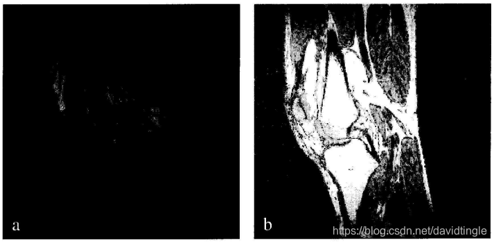
Figure 1. Example of contrast enhancement using histogram equalization.(a) The original image, an image of a human knee obtained with Magnetic Resonance Imaging. (b) Result of histogram equalization.
图1. 使用直方图均衡化增强对比度的例子。(a)原始图像,磁共振成像得到的人体膝盖图像。(b)直方图均衡化结果。
Adaptive Histogram Equalization (AHE)
Since our eyes adapt to the local context of images to evaluate their contents, it makes sense to optimize local image contrast(Pizer et al. 1987). To accomplish this, the image is divided in a grid of rectangular contextual regions in which the optimal contrast must be calculated. The optimal number of contextual regions depneds on the type of imput image, and its determination requires some experimentation. Division of the image into 8 x 8 contextual regions usually gives good results; this implies 64 contextual regions of size 64 x 64 when AHE is performed on a 512 x 512 image.
自适应直方图均衡化(AHE)
由于我们的眼睛适应于通过图像的局部上下文来评估其内容,因此优化局部图像对比度是有意义的(Pizer et al. 1987)。为了实现这一点,图像被分割成一个矩形上下文子区域(以下简称子区域)网格,其中最优对比度必须计算。最佳子区域数取决于输入图像的类型,确定最佳子区域数需要实验。通常将图像分割为8×8的子区域网格可以得到较好的效果; 比如:当使用AHE处理一个512 x 512的图像时,(8x8子区域网格)意味着整幅图像共计有64个大小为64 x 64的子区域。
For each of these contextual region, the histogram of the contained pixels is calculated. Calculation of the corresponding cumulative histograms results in a gray-level assignment table that optimizes contrast in each of the contextual regions, essentially a histogram equalization based on local image data.
对于每个子区域需计算其所包含像素的直方图。计算相应的累积直方图,得到一个对应每个子区域的优化对比度的灰度级分配表,本质上是基于局部图像数据的直方图均衡化。
To avoid visibility of region boundaries, a bilinear interpolation scheme is used(see Figure 2).
为了避免区域边界可见,使用了双线性插值方案(见图2)。
Applying adaptive histogram equalization on the image in Figure 1a results in the image that can be found in figure 2b. Although the contrast of the relevant structures in the knee is largely improved, the most striking feature of the image is the backgraound noise that has become visible. Although one can argue that AHE does what it is supposed to do -- optimal presentation of information present in the image -- noise present in AHE images turens out to be a major drawback of the method.
对图1a中的图像进行自适应直方图均衡化,得到的图像如图2b所示。虽然膝关节相关结构的对比度得到了很大的改善,但图像最显著的特征是背景噪声变得可见。尽管有人会说,AHE做了它应该做的事情——图像中呈现的信息的最佳呈现——但AHE图像中的噪声将成为该方法的一个主要缺点。
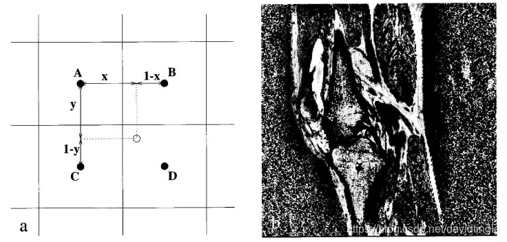
Figure 2. Subdivision and interpolation scheme used with adaptive histogram equalizationg and a typical result of AHE.(a) The gray-level assignment at the sample position, indicated by a white dot, is derived from the gray-value distributions in the surrounding contextural regions.The points A, B, C, and D form the center of the relevent contextual regions; region-specific gray-level mappings(gA(s), gB(s), gC(s), gD(s)) are based on the histogram of the pixels contained. Assuming that the original pixel intensity at the sample point is s. its new gray value is calculated by bilinear interpolation of the gray-level mappings that were calculated for each of the surrounding contextual regions; s' = (1 - y)((1-x)gA(s) + xgB(s)) + y((1-x)gC(s) + xgD(s)) where x and y are normalized distances with repect to the point A. at edges and corners, a slightly different interpolation scheme is used. (b) Result of AHE using 8 x 8 contextual regions applied on the image in Figure 1a. Although structures in the knee can be better distinguished, the overall appearance of the image suffers due to noise enhancement.
图2. 采用自适应直方图均衡化的细分和插值方案,以及一个AHE的典型结果。
(a)白点表示的样本位置的灰度分配来自于周围子区域的灰度分布。点A、点B、点C、点D构成相关子区域的中心;特定区域的灰度级映射(gA(s)、gB(s)、gC(s)、gD(s))基于所包含像素的直方图。假设样本点处的原始像素强度为s,其新的灰度值通过对每个周边背景区域计算的灰度级映射的双线性插值计算得到;s' = (1- y)((1-x)gA(s) + xgB(s)) + y((1-x)gC(s) + xgD(s)),其中x和y是对应于a点的归一化距离。
(b)在图1a图像上应用8×8个子区域的AHE结果。虽然膝盖的结构可以更好的区分,但图像的整体呈现受到噪声增强的影响。
Contrast Limited Adaptive Histogram Equalization (CLAHE)
The noise problem associated with AHE can be reduced by limiting contrast enhancement specifically in homogeneous areas. These areas can be characterized by a high peak in the histogram associated with the contextual regions since many pixels fall inside the same gray range. With CLAHE, the slope associated with the gray-level assignment scheme is limited; this can be accomplished by allowing only a maximum number of pixels in each of the bins associated with local histograms. After clipping the histogram, the pixels that were clipped are equally redistributed over the whole histogram to keep the total histogram count idential(see Figure 3).
与AHE相关的噪声问题可以通过限制对比度增强来降低,特别是在均匀区域。由于许多像素都在同一灰度范围内,因此这些区域可以通过与子区域相关的直方图中的一个峰值来表征。利用CLAHE,与灰度级分配方案相关的斜率是有限的;这可以通过在与局部直方图关联的每个容器中只允许最大像素数来实现。在裁剪直方图之后,被裁剪的像素在整个直方图上均匀地重新分布,以保持直方图总数的一致性(见图3)。
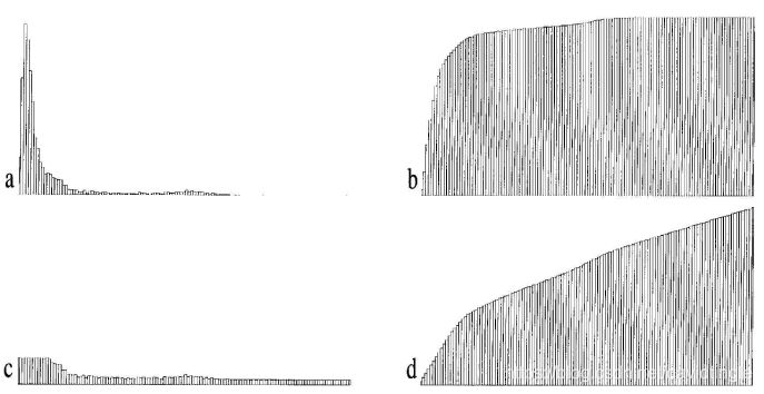
Figure3. Principle of contrast limiting as used with CLAHE. (a) Histogram of a contextual region containing many background pixels. (b) Calculated cumulative histogram; when used as a gray-level mapping, many bins are wasted for visualization of backgraound noise. (c) Clipped histogram obtained using a clip limit of three. Excess pixels are redistributed through the histogram. (d) Cumulative clipped histogram; its maximum slope (equal to the contrase enhancement obtained) is equal to the clip limit.
图3。CLAHE中使用的对比度限制原理。(a)包含许多背景像素的子区域的直方图。(b)计算的累积直方图;当用作灰度级映射时,许多容器会浪费在背景噪声的可视化上。(c)使用夹限为3的剪裁直方图。剪裁后多余的像素在直方图上重新分布。(d)累加剪裁直方图;其最大斜率(等于所得的对比度增强)等于夹限值。
The clip limit (or contrast factor) is defined as a multiple of the average histogram contents. With a low factor, the maximum slop of local histograms will be low and therefore result in limited contrast enhancement. A factor of one prohibits contrast enhancement (giving the original image); redistribution of histogram bin values can be avoided by using a very high clip limit(one thousand or higher), which is equivalent to the AHE technique.
剪裁限制(以下简称夹限)(或对比度因子)定义为平均直方图内容的倍数。当因子较低时,局部直方图的最大斜率较低,对比度增强有限。若需要阻止对比度增强(给出原始图像),这是一种方法。可以通过使用一个非常高的剪裁限制(1000或更高)来避免直方图bin值的重新分配,这相当于AHE技术。
Figure4 shows two examples of contrast enhancement using CLAHE; although the image at the right was CLAHE processed using a high clip limit, image noise is still acceptable;
图4显示使用CLAHE增强对比度的两个示例;虽然右边的图像是使用较高的夹限值,但图像噪声仍然可以接受;
The main advantages of the CLAHE transform as presented in this Gem are the modest computational requirements, its ease of use (requiring only one parameter; the clip limit), and its excellent results on most image.
本宝宝文中所提出的CLAHE转换主要优点是计算需求适中,容易使用(只需要一个参数:夹限值),以及处理大多数图像效果优异。
CLAHE does have disadvantages. Since the method is aimed at optimizing contrast, there is no 1 to 1 relationship between the gray value of the original image and the CLAHE processed result; consequently, CLAHE images are not suited for quantitative measurements that rely on a physical meaning of image intensity. A more serious problem are artifacts that sometimes occur when high-intensity gradients are present; see (Cromartie and Pizer 1991) for an explanation of these artifacts and a possible (but computationally expensive) solution. A detailed overview of AHE and other histogram equalization methods can be found in (Gauch 1992).
CLAHE确实有缺点。由于该方法旨在优化对比度,原始图像的灰度值与CLAHE处理结果之间不存在1对1的关系;因此,CLAHE图像不适合依赖于图像密度的物理意义的定量测量。更严重的问题是,当存在高密度梯度时会出现伪影;参见(Cromartie and Pizer 1991)对伪影的解释和一个可能的(但计算上高代价的)解决方案。AHE和其他直方图均衡化方法的详细概述见(Gauch 1992)。
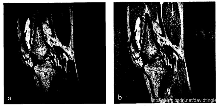
Figure 4. Result of CLAHE applied on the image in Figure 1a. (a) CLAHE with clip limit 2. (b) CLAHE with clip limit 10.Both image were obtained using 8 x 8 contextural regions.
图4. CLAHE应用于图1a图像的结果。(a)CLAHE夹限值为2 (b)CLAHE夹限值为10。两幅图像都是使用8×8的子区域获得的。
Implementation
Since CLAHE has its roots in medical imaging, the earlier CLAHE implementations assumed 16-bit image pixels, since medical scanners often generate 12-bit images. This implementation is a rewrite of a K&R C version written more than five years ago; it is now Ansi-C as well as C++ compliant and can also process 8-bit images.
For a 512 x 512 image, this implementation of CLAHE requires less than a second on an HP 9000/720 workstation when 8 x 8 contextual regions are used.
实现
由于CLAHE源于医学成像,医学扫描仪一般生成12位的图像, 所以早期的CLAHE实现假定图像像素为16位。本文的实现是对五年多前编写的K&R C版本的重写; 它现在是Ansi-C和c++兼容的,并且可以处理8位图像。
对512 x 512的图像,当使用8 x 8子区域时,在HP 9000/720工作站上CLAHE的执行不到一秒。
/*
 * ANSI C code from the article
 * "Contrast Limited Adaptive Histogram Equalization"
 * by Karel Zuiderveld, karel@cv.ruu.nl
 * in "Graphics Gems IV", Academic Press, 1994
 *
 *
 *  These functions implement Contrast Limited Adaptive Histogram Equalization.
 *  The main routine (CLAHE) expects an input image that is stored contiguously in
 *  memory;  the CLAHE output image overwrites the original input image and has the
 *  same minimum and maximum values (which must be provided by the user).
 *  This implementation assumes that the X- and Y image resolutions are an integer
 *  multiple of the X- and Y sizes of the contextual regions. A check on various other
 *  error conditions is performed.
 *
 *  #define the symbol BYTE_IMAGE to make this implementation suitable for
 *  8-bit images. The maximum number of contextual regions can be redefined
 *  by changing uiMAX_REG_X and/or uiMAX_REG_Y; the use of more than 256
 *  contextual regions is not recommended.
 *
 *  The code is ANSI-C and is also C++ compliant.
 *
 *  Author: Karel Zuiderveld, Computer Vision Research Group,
 *	     Utrecht, The Netherlands (karel@cv.ruu.nl)
 */

#ifdef BYTE_IMAGE
typedef unsigned char kz_pixel_t;    /* for 8 bit-per-pixel images */
#define uiNR_OF_GREY (256)
#else
typedef unsigned short kz_pixel_t;   /* for 12 bit-per-pixel images (default) */
# define uiNR_OF_GREY (4096)
#endif

/******** Prototype of CLAHE function. Put this in a separate include file. *****/
int CLAHE(kz_pixel_t *pImage, unsigned int uiXRes, unsigned int uiYRes, kz_pixel_t Min,
          kz_pixel_t Max, unsigned int uiNrX, unsigned int uiNrY,
          unsigned int uiNrBins, float fCliplimit);

/*********************** Local prototypes ************************/
static void ClipHistogram(unsigned long *, unsigned int, unsigned long);
static void MakeHistogram(kz_pixel_t *, unsigned int, unsigned int, unsigned int,
                          unsigned long *, unsigned int, kz_pixel_t *);
static void MapHistogram(unsigned long *, kz_pixel_t, kz_pixel_t,
                         unsigned int, unsigned long);
static void MakeLut(kz_pixel_t *, kz_pixel_t, kz_pixel_t, unsigned int);
static void Interpolate(kz_pixel_t *, int, unsigned long *, unsigned long *,
                        unsigned long *, unsigned long *, unsigned int, unsigned int, kz_pixel_t *);

/**************	 Start of actual code **************/
#include <stdlib.h>          /* To get prototypes of malloc() and free() */

const unsigned int uiMAX_REG_X = 16;      /* max. # contextual regions in x-direction */
const unsigned int uiMAX_REG_Y = 16;      /* max. # contextual regions in y-direction */


/************************** main function CLAHE ******************/
int CLAHE(kz_pixel_t *pImage, unsigned int uiXRes, unsigned int uiYRes,
          kz_pixel_t Min, kz_pixel_t Max, unsigned int uiNrX, unsigned int uiNrY,
          unsigned int uiNrBins, float fCliplimit)

/*   pImage - Pointer to the input/output image
 *   uiXRes - Image resolution in the X direction
 *   uiYRes - Image resolution in the Y direction
 *   Min - Minimum greyvalue of input image (also becomes minimum of output image)
 *   Max - Maximum greyvalue of input image (also becomes maximum of output image)
 *   uiNrX - Number of contextial regions in the X direction (min 2, max uiMAX_REG_X)
 *   uiNrY - Number of contextial regions in the Y direction (min 2, max uiMAX_REG_Y)
 *   uiNrBins - Number of greybins for histogram ("dynamic range")
 *   float fCliplimit - Normalized cliplimit (higher values give more contrast)
 * The number of "effective" greylevels in the output image is set by uiNrBins; selecting
 * a small value (eg. 128) speeds up processing and still produce an output image of
 * good quality. The output image will have the same minimum and maximum value as the input
 * image. A clip limit smaller than 1 results in standard (non-contrast limited) AHE.
 */
{
    unsigned int uiX, uiY;        /* counters */
    unsigned int uiXSize, uiYSize, uiSubX, uiSubY; /* size of context. reg. and subimages */
    unsigned int uiXL, uiXR, uiYU, uiYB;  /* auxiliary variables interpolation routine */
    unsigned long ulClipLimit, ulNrPixels; /* clip limit and region pixel count */
    kz_pixel_t *pImPointer;        /* pointer to image */
    kz_pixel_t aLUT[uiNR_OF_GREY];      /* lookup table used for scaling of input image */
    unsigned long *pulHist, *pulMapArray; /* pointer to histogram and mappings*/
    unsigned long *pulLU, *pulLB, *pulRU, *pulRB; /* auxiliary pointers interpolation */

    if (uiNrX > uiMAX_REG_X)
        return -1;                         /* # of regions x-direction too large */

    if (uiNrY > uiMAX_REG_Y)
        return -2;                         /* # of regions y-direction too large */

    if (uiXRes % uiNrX)
        return -3;                    /* x-resolution no multiple of uiNrX */

    if (uiYRes % uiNrY)
        return -4;                    /* y-resolution no multiple of uiNrY */

    if (Max >= uiNR_OF_GREY)
        return -5;                         /* maximum too large */

    if (Min >= Max)
        return -6;                /* minimum equal or larger than maximum */

    if (uiNrX < 2 || uiNrY < 2)
        return -7;                /* at least 4 contextual regions required */

    if (fCliplimit == 1.0)
        return 0;                 /* is OK, immediately returns original image. */

    if (uiNrBins == 0)
        uiNrBins = 128;           /* default value when not specified */

    pulMapArray = (unsigned long *)malloc(sizeof(unsigned long) * uiNrX * uiNrY * uiNrBins);
    if (pulMapArray == 0)
        return -8;                /* Not enough memory! (try reducing uiNrBins) */

    uiXSize = uiXRes / uiNrX;
    uiYSize = uiYRes / uiNrY;    /* Actual size of contextual regions */
    ulNrPixels = (unsigned long)uiXSize * (unsigned long)uiYSize;

    if (fCliplimit > 0.0)        /* Calculate actual cliplimit	 */
    {
        ulClipLimit = (unsigned long) (fCliplimit * (uiXSize * uiYSize) / uiNrBins);
        ulClipLimit = (ulClipLimit < 1UL) ? 1UL : ulClipLimit;
    }
    else
        ulClipLimit = 1UL << 14;      /* Large value, do not clip (AHE) */

    MakeLut(aLUT, Min, Max, uiNrBins);    /* Make lookup table for mapping of greyvalues */
    /* Calculate greylevel mappings for each contextual region */
    for (uiY = 0, pImPointer = pImage; uiY < uiNrY; uiY++)
    {
        for (uiX = 0; uiX < uiNrX; uiX++, pImPointer += uiXSize)
        {
            pulHist = &pulMapArray[uiNrBins * (uiY * uiNrX + uiX)];
            MakeHistogram(pImPointer, uiXRes, uiXSize, uiYSize, pulHist, uiNrBins, aLUT);
            ClipHistogram(pulHist, uiNrBins, ulClipLimit);
            MapHistogram(pulHist, Min, Max, uiNrBins, ulNrPixels);
        }

        pImPointer += (uiYSize - 1) * uiXRes;     /* skip lines, set pointer */
    }

    /* Interpolate greylevel mappings to get CLAHE image */
    for (pImPointer = pImage, uiY = 0; uiY <= uiNrY; uiY++)
    {
        if (uiY == 0)                 /* special case: top row */
        {
            uiSubY = uiYSize >> 1;
            uiYU = 0;
            uiYB = 0;
        }
        else
        {
            if (uiY == uiNrY)             /* special case: bottom row */
            {
                uiSubY = (uiYSize + 1) >> 1;
                uiYU = uiNrY - 1;
                uiYB = uiYU;
            }
            else                  /* default values */
            {
                uiSubY = uiYSize;
                uiYU = uiY - 1;
                uiYB = uiYU + 1;
            }
        }

        for (uiX = 0; uiX <= uiNrX; uiX++)
        {
            if (uiX == 0)             /* special case: left column */
            {
                uiSubX = uiXSize >> 1;
                uiXL = 0;
                uiXR = 0;
            }
            else
            {
                if (uiX == uiNrX)     /* special case: right column */
                {
                    uiSubX = (uiXSize + 1) >> 1;
                    uiXL = uiNrX - 1;
                    uiXR = uiXL;
                }
                else              /* default values */
                {
                    uiSubX = uiXSize;
                    uiXL = uiX - 1;
                    uiXR = uiXL + 1;
                }
            }

            pulLU = &pulMapArray[uiNrBins * (uiYU * uiNrX + uiXL)];
            pulRU = &pulMapArray[uiNrBins * (uiYU * uiNrX + uiXR)];
            pulLB = &pulMapArray[uiNrBins * (uiYB * uiNrX + uiXL)];
            pulRB = &pulMapArray[uiNrBins * (uiYB * uiNrX + uiXR)];
            Interpolate(pImPointer, uiXRes, pulLU, pulRU, pulLB, pulRB, uiSubX, uiSubY, aLUT);
            pImPointer += uiSubX;         /* set pointer on next matrix */
        }

        pImPointer += (uiSubY - 1) * uiXRes;
    }

    free(pulMapArray);                    /* free space for histograms */
    return 0;                         /* return status OK */
}

/*****************************************************************************
 * Function:             ClipHistogram
 * Description:          TODO
 * Input:                TODO
 * Output:               N/A
 * Return:
 *   OK:                    Successful
 *   ERROR:                 Failed
 ******************************************************************************/
void ClipHistogram(unsigned long *pulHistogram, unsigned int
                   uiNrGreylevels, unsigned long ulClipLimit)

/* This function performs clipping of the histogram and redistribution of bins.
 * The histogram is clipped and the number of excess pixels is counted. Afterwards
 * the excess pixels are equally redistributed across the whole histogram (providing
 * the bin count is smaller than the cliplimit).
 */
{
    unsigned long *pulBinPointer, *pulEndPointer, *pulHisto;
    unsigned long ulNrExcess, ulUpper, ulBinIncr, ulStepSize, i;
    long lBinExcess;

    ulNrExcess = 0;
    pulBinPointer = pulHistogram;
    for (i = 0; i < uiNrGreylevels; i++)   /* calculate total number of excess pixels */
    {
        lBinExcess = (long) pulBinPointer[i] - (long) ulClipLimit;
        if (lBinExcess > 0)
            ulNrExcess += lBinExcess;                 /* excess in current bin */

    }

    ;

    /* Second part: clip histogram and redistribute excess pixels in each bin */
    ulBinIncr = ulNrExcess / uiNrGreylevels;          /* average binincrement */
    ulUpper = ulClipLimit - ulBinIncr;   /* Bins larger than ulUpper set to cliplimit */

    for (i = 0; i < uiNrGreylevels; i++)
    {
        if (pulHistogram[i] > ulClipLimit)
            pulHistogram[i] = ulClipLimit;                              /* clip bin */
        else
        {
            if (pulHistogram[i] > ulUpper)  /* high bin count */
            {
                ulNrExcess -= pulHistogram[i] - ulUpper;
                pulHistogram[i] = ulClipLimit;
            }
            else                /* low bin count */
            {
                ulNrExcess -= ulBinIncr;
                pulHistogram[i] += ulBinIncr;
            }
        }
    }

    while (ulNrExcess)     /* Redistribute remaining excess  */
    {
        pulEndPointer = &pulHistogram[uiNrGreylevels];
        pulHisto = pulHistogram;

        while (ulNrExcess && pulHisto < pulEndPointer)
        {
            ulStepSize = uiNrGreylevels / ulNrExcess;
            if (ulStepSize < 1)
                ulStepSize = 1;                   /* stepsize at least 1 */

            for (pulBinPointer = pulHisto; pulBinPointer < pulEndPointer && ulNrExcess;
                 pulBinPointer += ulStepSize)
            {
                if (*pulBinPointer < ulClipLimit)
                {
                    (*pulBinPointer)++;
                    ulNrExcess--;                 /* reduce excess */
                }
            }

            pulHisto++;   /* restart redistributing on other bin location */
        }
    }
}

/*****************************************************************************
 * Function:             MakeHistogram
 * Description:          TODO
 * Input:                TODO
 * Output:               N/A
 * Return:
 *   OK:                    Successful
 *   ERROR:                 Failed
 ******************************************************************************/
void MakeHistogram(kz_pixel_t *pImage, unsigned int uiXRes,
                   unsigned int uiSizeX, unsigned int uiSizeY,
                   unsigned long *pulHistogram,
                   unsigned int uiNrGreylevels, kz_pixel_t *pLookupTable)

/* This function classifies the greylevels present in the array image into
 * a greylevel histogram. The pLookupTable specifies the relationship
 * between the greyvalue of the pixel (typically between 0 and 4095) and
 * the corresponding bin in the histogram (usually containing only 128 bins).
 */
{
    kz_pixel_t *pImagePointer;
    unsigned int i;

    for (i = 0; i < uiNrGreylevels; i++)
        pulHistogram[i] = 0L;                                  /* clear histogram */

    for (i = 0; i < uiSizeY; i++)
    {
        pImagePointer = &pImage[uiSizeX];
        while (pImage < pImagePointer)
            pulHistogram[pLookupTable[*pImage++]]++;

        pImagePointer += uiXRes;
        pImage = &pImagePointer[-(int)uiSizeX]; /* go to bdeginning of next row */
    }
}

/*****************************************************************************
 * Function:             MapHistogram
 * Description:          TODO
 * Input:                TODO
 * Output:               N/A
 * Return:
 *   OK:                    Successful
 *   ERROR:                 Failed
 ******************************************************************************/
void MapHistogram(unsigned long *pulHistogram, kz_pixel_t Min, kz_pixel_t Max,
                  unsigned int uiNrGreylevels, unsigned long ulNrOfPixels)

/* This function calculates the equalized lookup table (mapping) by
 * cumulating the input histogram. Note: lookup table is rescaled in range [Min..Max].
 */
{
    unsigned int i;
    unsigned long ulSum = 0;
    const float fScale = ((float)(Max - Min)) / ulNrOfPixels;
    const unsigned long ulMin = (unsigned long) Min;

    for (i = 0; i < uiNrGreylevels; i++)
    {
        ulSum += pulHistogram[i];
        pulHistogram[i] = (unsigned long)(ulMin + ulSum * fScale);
        if (pulHistogram[i] > Max)
            pulHistogram[i] = Max;
    }
}

/*****************************************************************************
 * Function:             MakeLut
 * Description:          TODO
 * Input:                TODO
 * Output:               N/A
 * Return:
 *   OK:                    Successful
 *   ERROR:                 Failed
 ******************************************************************************/
void MakeLut(kz_pixel_t *pLUT, kz_pixel_t Min, kz_pixel_t Max, unsigned int uiNrBins)

/* To speed up histogram clipping, the input image [Min,Max] is scaled down to
 * [0,uiNrBins-1]. This function calculates the LUT.
 */
{
    int i;
    const kz_pixel_t BinSize = (kz_pixel_t) (1 + (Max - Min) / uiNrBins);

    for (i = Min; i <= Max; i++)
        pLUT[i] = (i - Min) / BinSize;
}

/*****************************************************************************
 * Function:             Interpolate
 * Description:          TODO
 * Input:                TODO
 * Output:               N/A
 * Return:
 *   OK:                    Successful
 *   ERROR:                 Failed
 ******************************************************************************/
void Interpolate(kz_pixel_t *pImage, int uiXRes, unsigned long *pulMapLU,
                 unsigned long *pulMapRU, unsigned long *pulMapLB, unsigned long *pulMapRB,
                 unsigned int uiXSize, unsigned int uiYSize, kz_pixel_t *pLUT)

/* pImage      - pointer to input/output image
 * uiXRes      - resolution of image in x-direction
 * pulMap*     - mappings of greylevels from histograms
 * uiXSize     - uiXSize of image submatrix
 * uiYSize     - uiYSize of image submatrix
 * pLUT	       - lookup table containing mapping greyvalues to bins
 * This function calculates the new greylevel assignments of pixels within a submatrix
 * of the image with size uiXSize and uiYSize. This is done by a bilinear interpolation
 * between four different mappings in order to eliminate boundary artifacts.
 * It uses a division; since division is often an expensive operation, I added code to
 * perform a logical shift instead when feasible.
 */
{
    const unsigned int uiIncr = uiXRes - uiXSize; /* Pointer increment after processing row */
    kz_pixel_t GreyValue;
    unsigned int uiNum = uiXSize * uiYSize;                     /* Normalization factor */

    unsigned int uiXCoef, uiYCoef, uiXInvCoef, uiYInvCoef, uiShift = 0;

    if (uiNum & (uiNum - 1))   /* If uiNum is not a power of two, use division */
        for (uiYCoef = 0, uiYInvCoef = uiYSize; uiYCoef < uiYSize;
             uiYCoef++, uiYInvCoef--, pImage += uiIncr)
        {
            for (uiXCoef = 0, uiXInvCoef = uiXSize; uiXCoef < uiXSize;
                 uiXCoef++, uiXInvCoef--)
            {
                GreyValue = pLUT[*pImage]; /* get histogram bin value */
                *pImage++ = (kz_pixel_t) ((uiYInvCoef * (uiXInvCoef * pulMapLU[GreyValue]
                                                         + uiXCoef * pulMapRU[GreyValue])
                                           + uiYCoef * (uiXInvCoef * pulMapLB[GreyValue]
                                                        + uiXCoef * pulMapRB[GreyValue])) / uiNum);
            }
        }

    else               /* avoid the division and use a right shift instead */
    {
        while (uiNum >>= 1)
            uiShift++;                     /* Calculate 2log of uiNum */

        for (uiYCoef = 0, uiYInvCoef = uiYSize; uiYCoef < uiYSize;
             uiYCoef++, uiYInvCoef--, pImage += uiIncr)
        {
            for (uiXCoef = 0, uiXInvCoef = uiXSize; uiXCoef < uiXSize;
                 uiXCoef++, uiXInvCoef--)
            {
                GreyValue = pLUT[*pImage]; /* get histogram bin value */
                *pImage++ = (kz_pixel_t)((uiYInvCoef * (uiXInvCoef * pulMapLU[GreyValue]
                                                        + uiXCoef * pulMapRU[GreyValue])
                                          + uiYCoef * (uiXInvCoef * pulMapLB[GreyValue]
                                                       + uiXCoef * pulMapRB[GreyValue])) >> uiShift);
            }
        }
    }
}
Bibliography
参考文献
(Cromartie and Pizer 1991) R. Cromartie and S.M. Pizer. Edge-affected context for adaptive contrast enhancement. In A. C. S. Colchester and D. J. Hawkes, editors, Proceedings of the XIIth International Meeting on Information Processing in Medical Imaging: Lecture Notes in Computer Science, pages 474-485, Springer-Verlag, Berlin, 1991.
(Gauch 1992) J. M. Gauch. Investigations of image contrast space defined by variations on histogram equalization. CVGIP: Graphical Models and Image Processing, 54(4):269-280, July 1992.
(Jain 1989) A. K. Jain. Fundamentals of digital image processing. Prentice Hall, Englewood Cliffs, NJ, 1989.
(Pizer et al. 1987) S. M. Pizer, E. P. Amburn, J. D. Austin, R. Cromartie, A. Geselowitz, B. ter Haar Romeny, J. B. Zimmerman, and K. Zuiderveld. Adaptive histogram equalization and its variations. Computer Vision, Graphics, and Image Processing, 39:355-368, 1987
(Rosenman et al. 1993)J. Rosenman, C.A. Roe, R. Cromartie, K.E. Muller, and S. M. Pizer. Portal film enhancement: Technique and clinical utility. Int. J. Radiat. Oncol. Biol. Physics, pages 333-338, 1993.


 1518
1518

 被折叠的 条评论
为什么被折叠?
被折叠的 条评论
为什么被折叠?
 到【灌水乐园】发言


