6D姿态估计从0单排——看论文的小鸡篇——Learning 6D Object Pose Estimation using 3D Object Coordinates...

这篇文章内容是真的多，而且大段的文字，图和公式都很少，看起来很枯燥。。。说白了就是把整个模型拆成555的125个部分，这样一个像素点都扔进去随机森林里面训练和匹配，然后查出来他最可能的类别和在一个模型中位置。就一如他的开头这句话：The key new concept is a representation in form of a dense 3D object coordinate labelling paired with a dense class labelling.（关键的新概念就是将一个稠密的3D模型坐标标记搭配稠密的类别标记组建而成的表达方式）
使用LHCF（Latent-Class Hough Forests）：拆分模型成多个patch、用patch去匹配，并且使用random forest加速匹配速度，从而更快地找到对应的位置
The key new concept is a representation in form of a dense 3D object coordinate labelling paired with a dense class labelling.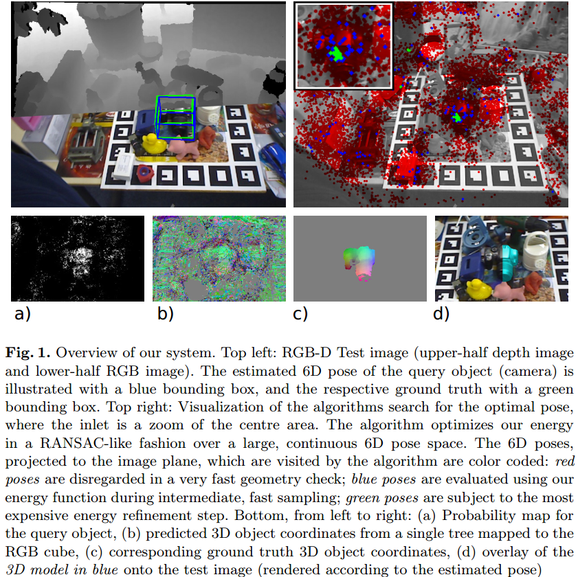

template-based techniques have in our view two fundamental shortcomings. Firstly, they match the complete template to a target image, i.e. encode the object in a particular pose with one "global" feature. In contrast to this, sparse feature-based representations for textured objects are "local" and hence such systems are more robust with respect to occlusions. Secondly, it is an open challenge to make template-based techniques work for articulated or deformable object instances, as well as object classes, due to the growing number of required templates.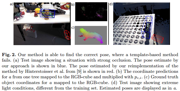

Work：a new approach that has the benefits of local feature-based object detection techniques and still achieves results that are superior to templatebased techniques for texture-less object detection.
Advantanges: 1. use for textured and texture-less object 2. use for rigid and non-rigid object 3. robustness with respect to occlusions 4. robust to occlusions.
use of a new representation in form of a joint dense 3D object coordinate and object class labelling

1. Random forest
   Use a single decision forest to classify pixels from an RGB-D image. A decision forest is a set \(T\) of decision trees \(T^j\). Pixels of an image are classified by each tree \(T^j\) and end up in one of the tree’s leafs \(l^j\). Our forest allows us to gain information about which object \(c\in C\) the pixel \(i\) might belong to, as well as what might be its position on this object. a pixel's position on the object is denote by \(y_i\) and referred to as the pixel's object coordinate. Each leaf \(l^j\) stores a distribution over possible object affiliations \(p(c|l^j)\), as well as a set of object coordinates \(y_c(l^j)\) for each possible object affiliation \(c\). \(y_c(l^j)\) will be referred to as coordinate prediction
   Design and Training of the Forest: quantized the continuous distributions \(p(y|c)\) into 555 = 125 discrete bins and an additional bin for a background class. This has potentially \(125|C|+1\) labels, for \(|C|\) object instances and background, though many bins are empty. As a node split objective that deals with both our discrete distributions, we use the information gain over the joint distribution.
   Use the features which consider depth or color differences from pixels in the vicinity of pixel \(i\) and capture local patterns of context to split objective in the tree splits. Each object is segmented for training.
   For training, we use randomly sampled pixels from the segmented object images and a set of RGB-D background images. we push training pixels from all objects through the tree and record all the continuous locations \(y\) for each object \(c\) at each leaf. And then run mean-shift with a Gaussian kernel. Use the top mode as prediction \(y_c(l^j)\) and store it at the leaf. Store at each leaf the percentage of pixels coming from each object \(c\) to approximate the distribution of object affiliations \(p(c|l^j)\) at the leaf and store the percentage of pixels from the background set that arrived at \(l^j\), and refer to it as \(p(bg|l^j)\).
   Using the Forest:
   After training, we push all pixels in an RGB-D image through every tree of the forest, thus associating each pixel \(i\) with a distribution \(p(c|l^j_i)\) and prediction \(y_c(l^j_i)\) for each tree \(j\) and each object \(c\). Here \(l_i^j\) is the leaf outcome of pixel \(i\) in the tree \(j\). The leaf outcome of all trees for a pixel \(i\). Summarized outcome is \(I_i = (l_i^1,...,l_i^j,...,l_i^{|T|})\). And the image is summarized in \(L = (I_1,...I_n)\). We calculate a number \(p_{c,i}\) by combining the \(p(c|l_i^j)\). The number can be seen as the approximate probability \(p(c|l_i)\) of the \(i\) pixel and object \(c\). And then we calculate the probability as: \(p_{c,i} = \frac{\prod^{|T|}_{j=1}p(c|l^j_i)}{\prod^{|T|}_{j=1}p(bg|l_i^j) + \sum_{\vec{c}\in C}\prod^{|T|}_{j=1}p(\vec{c}|l^j_i)}\)
2. Energy Function
   
   depth \(D = (d1,...d_n)\) and the result of the forest \(L=(I_1,...I_n)\)
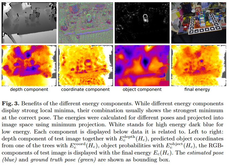
   The energy function is based on three components: \(\vec{E}_c(H_c) = \lambda^{depth}E_c^{depth}(H_c) + \lambda^{coord}E_c^{coord}(H_c) +\lambda^{obj}E_c^{obj}(H_c)\), H_c is the pose, \(E_c^{depth}(H)\) punished deviations between the observed and ideal rendered depth images, the \(E_c^{coord}(H)\) and the \(E_c^{obj}(H)\) punish the deviations from the predictions of the forest.
   Depth Component: \(E_c^{depth}(H_c) = \frac{\sum_{i \in M_c^D(H_c)}f(d_i, d_i^*(H_c))}{\left|M_c^D(H_c)\right|}\), where the \(M_c^D(H_c)\) is the set of pixels belonging to object \(c\), \(d_i\) is Pixels with no depth observation, \(d^∗_i(H_c)\) the depth at pixel \(i\) of our recorded 3D model for object \(c\) rendered with pose \(H_c\). Error function: \(f(d_i, d_i^*(H)) = min(\left\|x(d_i)-x(d_i^*(H))\right\|, \tau_d)/\tau_d\), \(x(d_i)\) denotes the 3D coordianates in camera system derived from the depth \(d_i\). The denominator in the definition normalizes the depth component to make it independent of the object’s distance to the camera ( \(\tau\)找了一圈没找到定义。。。感觉是距离？下角标d貌似没什么特别意思)
   Object Component: punishes pixels inside the ideal segmentation \(M_c^D\) which are, according to the forest, unlikely to belong to the object. It is \(E_c^{obj}(H_c)=\frac{\sum_{i\in M_c^D(H_c)\sum^{\left|T\right|}_{j=1}-\log p(c|l_i^j)}}{\left|M_c^D(H_c)\right|}\)
   Coordinate Component: punishes deviations between the object coordinates \(y_c(l_i^j)\) predicted by the forest and ideal object coordinates \(y_{i,c}(H_c)\) derived from a rendered image. It is : \(E_c^coord(H_c) = \frac{\sum_{i\in M_c^L(H_c)}\sum_{j=1}^{\left|T\right|}g(y_c(l^j_i), y_{i,c}(H_c))}{\left|M_c^L(H_c)\right|}\), \(M^L_c(H_c)\) is the set of pixels belonging to the object \(c\) excluding pixels with no depth observation \(d_i\) and pixels where \(p_{c,i} < \tau_{pc}\)(看这个定义的话，感觉\(\tau\)应该是一个阈值？). \(y_{i,c}(H_c)\) denotes the coordinates in the object space at pixel \(i\) of our 3D model for object \(c\) rendered with pose \(H_c\). We again use a robust function: \(g(y_c(l^j_i), y_{i,c}(H_c)) = min(\left\|y_c(l_i^j)-y_{i,c}(H_c)\right\|^2, \tau_y)/\tau_y\)
   Final function: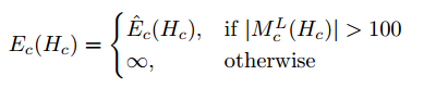
   
3. Optimization
   Sampling os a Pose Hypothesis We first draw a single pixel \(i_1\) from the image using a weight proportional to the previously calculated \(p_{c,i}\) each pixel \(i\). We draw two more pixels \(i_2\) and \(i_3\) from a square window around \(i_1\) using the same method. The width is calculated from the diameter of the object and the observed depth value \(d_{i_1}\) od the pixel \(w = f\delta_c/d_i\) where \(f = 575.816\) pixels. We randomly choose a tree index \(j_1, j_2, j_3\) for each pixel. we use the Kabsch algorithm to calculate the pose hypothesis \(H_c\) from the three outcome. And then use the \(H_c\) to calculate the Euclidean distance error. We accept a pose \(H_c\) only if none of the three distances is larger than 5% of object. The process repeat until a fixed number of 210 hypotheses are accepted.
   Refinement We refine the top 25 accepted hypotheses. To refine the pose, we iterate over set of pixels \(M_c^D(H_c)\) supposedly belonging to the object \(c\) as done for energey calculation. For every pixel, we calculate the error for all trees \(j\). Let \(\vec{j}\) be the tree with the smallest error for pixel \(i\). And every pixel where \(e_{i,\vec{j}}(H_c)<20mm\) is considered an inlier. We store the correspondece \((x(i_1), y_c(l_i^j))\) for all inlier pixels and reestimate with Kabsch algorithm. Repeate until the energy function no longer decreases, the nmber of inlier pixels drops below 3, or 100 iterations is reached.
   Final Estimate THe pose hypothesis with the lowest energy after refinement is chosen as final estimate.

转载于:https://www.cnblogs.com/LeeGoHigh/p/10482880.html