6D姿态估计从0单排——看论文的小鸡篇——Detection and Fine 3D Pose Estimation of Texture-less Objects in RGB-D Images...

这是我现在做的最长的一篇笔记了。。。感觉挺有意思的这个，首先是用一个流动视窗搜索全图，然后删除大部分没有搜寻物体的候选，余下的部分使用启发式的操作得出特征信息然后和模板的hash匹配看那些模板比较有可能，得出了全部的模板后然后对每个模板的物体直径、法向量、梯度、深度、色彩对比得到候选，候选进一步得到pose，再对pose经行梯度、边框、法向量的评估，最后用PSO的办法收敛到最优解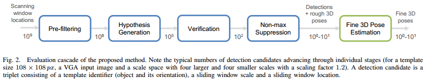

The proposed method address the excessive computational complexity of sliding window approaches and achieves high efficiency by employing a cascade-style evaluation of window locations. Fast filtering is performed first, rejecting quickly most of the locations by simple salience check. For each remaining locations by a simple salience check. For each remaining location, candidate templates are obtained by efficient voting procedure based on hashing measurements sampled on a regular grid. This makes the complexity of the method sub-linear in the total number of known objects. The candidate templates are then verified by matching feature points in different modalities. Each template is associated with a training-time pose i.e. a 3D rotation and distance to the camera reference frame origin. Therefore, a successful match against a template provides a rough estimate of the object's 3D location and orientation. As a final step, a stochastic, population-based optimization scheme is applied to refine the pose by fitting a 3D model of the detected object to the input depth map.
Detection Of Texture-less Objects
Detection of objects in an input RGB-D image is based on a sliding window approach, operating on a scale pyramid built from image. \(L\) is the set of all tested locations. The number of locations \(\left|L\right|\) is a function of image resolution. The objects are represented with a set \(T\). Template is associated with the object ID, the training distance \(Z_t\) and object orientation \(R_0\). In every window \(w_l\), \(l = (x,y,s), I\in L\) need to be tested against every template.

1. Pre-filtering of Window Locations
   Our objectness measure is based on the number of depth-discontinuity edgels(edge pixel 边缘像素) within the window, and is computed with the aid of an integral image for efficiency. The edgels arise at pixels where the response of the Sobel operator, computed over the depth image, is above a threshold \(\theta_e\), which is set to 30% of the physical diameter of the smallest object in the database.
2. Hypothesis Generation
   A small subset of candidate templates is quickly identified for each image window that passed the objectness test. Up to \(N\) templates, which at least \(v\) votes, with the highest probabilities \(p_t(t|w_1), t\in T\) are retrieved. The procedure retrieves candidate templates from multiple trained hash tables which stored templates. Each hash table \(h\in H\) is indexed by a trained set \(M_h\) of measurements taken on the window \(w_1\) or template \(t\), discretized into a hash key. \(M_h\) is different for each table. The table cells contain lists of templates with the same key, the lists are then used to vote for the templates. A template can receive up to \(\left|H\right|\)
   Measurement sets \(M_h\) and their quantization: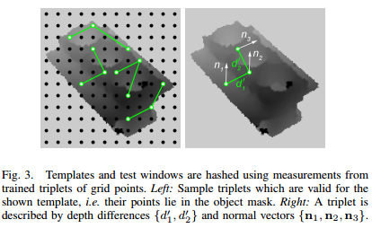
   
   A regular grid of 12*12 reference points is placed over the training template or sliding window. This yields 144 locations from which k-tuples are sampled. Each location is assigned with a depth \(d\) and a surface normal \(n\). A measurement set \(M_h\) is a vector consisting of \(k-1\) relative depth values and \(k\) normals, \(M_h=(d_{2h}-d_{1h}, d_{3h}-d_{1h}, ..., d_{kh}-d_{1h}, n_{1h}, ..., n_{kh})\). The relative depths \(d_{ih} − d_{1h}\) are quantized into 5 bins each, with the quantization boundaries learned from all the training templates to provide equal frequency binning. The normals are quantized to 8 discrete values based on their orientation.
   Training-time selection of measurement sets: multiple hash tables are built, which differ in the selection of the k-tuples drawn from the 144 reference points. The k-tuples can be chosen randomly. We first randomly generate a set of \(m, m >> \left|H\right|\), \(k\)-tuples and then retain the subset with the largest joint entropy of the quantized measurements.
3. Hypothesis Verification:
   The verification proceeds in a sequence of tests evaluating the following: 1. object size in relation to distance, 2. sampled surface normals, 3. sampled image gradients, 4. sampled depth map, 5. sampled color. Any failed test classifies the window as non-object - corresponding to either the background, or an object not represented by template - and subsequent tests are not evaluated.
   1 test: distance \(Z_e = Z_ts\), \(s\) is scale factor of the pyramid level and \(Z_t\) is the template's training distance. If the measured depth \(Z_w\) is within the \(\left|Z_e/\sqrt{f},Z_e*\sqrt{f}\right|\), where \(f\) is the discretization factor of the scale space, the depth is considered to be feasible.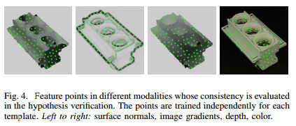
   
   2 & 3 test: verify orientation of normals and gradients at several feature points. The feature points for the surface normal orientation test are extracted at locations with locally stable orientation of normals. For the intensity gradient orientation test, the feature points are extracted at locations with large gradient magnitude.
   4 & 5 test: reuse the locations of feature points extracted for the surface normal test. In the depth test, difference d between the depth in the template and the depth in the window is calculated for each feature point. A feature point is matched if \(\left|d-d_m\right|<kD\), \(d_m\) is the median value of \(d\)s over all feature points, \(D\) is the physical object diameter, \(k\) is a coefficient. Pixel colors in test are compared in the HSV space.
   A template passes the test 2\3\4\5 if at least \(\theta_c\) of the feature points have a matching value within a small neighbourhood. A template that passed all tests is assigned a final score \(m = \sum_{i\in \{2,3,4,5\}c_i}\), \(c_i\)is the fraction of the matching feature points.
4. Non-maxima Suppression
   The score is calculated as \(r = m(a/s)\), where \(m\) is the verification score defined above, \(s\) is the detection scale, and \(a\) is the area of the object in the considered template.

Fine 3D Pose Estimation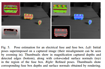

Candidate poses \(\{R_i, t_i\}\). Model \(M\) is comprised of an ordered set of 3D vertex points \(V\), the oriented bounding box \(B\) is computed using the eigenvectors of \(V\)'s covariance matrix. depth images \(S_i\). scoring function yields score \(o(i)\) which quantifies the similarity between each image \(S_i\) and the input using depth, edge and orientation cues. PSO is used to optimize the scoring function and find the pose whose rendered depth image is the most similar to the input one.

1. initialization
   To suppress sensor noise, the acquired depth image is median filtered with a 5 × 5 kernel and the result is retained as image \(D\). Surface normals for valid depth pixels are estimated by local least-squares plane fitting and stored in \(N\). Binary image \(E\) is computed from \(D\)/
2. Pose Hypotheses Rendering
   Candidate poses are parametrized relative to this initial pose, using a relative translation \(t_i\) and an “in place” rotation \(R_i\) about the centroid
   \(c\) of points in \(V\). Specifically, the model is first translated by \(−c\), rotated by \(R_i\), and translated back to place by \(c\). Rotation \(R_i\) is the product of primitive rotations about the
   3 axes: \(R_i = R_x(\theta_i)*R_y(\phi_i)*R_z(\omega_i)\). The transformation model point x undergoes is thus \(R_i*(x−c)+c+t_i\). To avoid repeated transformations, the initial and candidate poses are combined into the following: \(R_i*R_0*x + R_i*(t_0-c)+c+t_i\) The rotational component of candidate poses is parameterized using Euler angles whereas their translation is parameterized with Euclidean coordinates. At a fine level, rendering is parallelized upon the triangles of the rendered mesh. At a coarser level, multiple hypotheses are rendered simultaneously, with a composite image gathering all renderings.
3. Pose Hypotheses Evaluation
   A candidate pose is evaluated with respect to the extent to which it explains the input depth image.
   Depth values are directly compared between \(D\) and \(Si\) for pairs of pixels. For \(n\) pixel pairs, depth differences \(\delta_k\), are computed and the cumulative depth cost term is defined as: \(d_i = \sum_{k=1}^n1/(|\delta_k|+1)\) where \(|\delta_k|\) is set to 1 if greater than threshold \(d_T\). For the same \(n\) pairs of pixels, the cost due to surface normal differences is quantified as: \(u_i = \sum_{k=1}^n1/(|\gamma_k|+1)\) where \(|\gamma_k|\) is the angle between the two surface normals, provided by their dot product.
   Edge differences are aggregated in an edge cost using \(E\) and \(E_i\). Let m be the number of edgels of \(E_i\) within \(b\). For each such edgel \(j\), let \(\epsilon_j\) denote the distance from its closest edgel in \(D\) which is looked up from \(T\). The corresponding edge cost term is then: \(e_i=\sum^m_{j=1}1/(\epsilon_j+1)\)
   The similarity score \(o(i)=-d_i*e_i*u_i\) where the minus sign is used to ensure that optimal values correspond to minima. The objective function improves when more pixels in the rendered depth map closely overlap with the imaged surfaces in the input image.
   As no segmentation is employed, inaccurate pose hypotheses might cause the rendered object to be compared against pixels imaging background or occluding surfaces. To counter this, only pixels located within \(b\) are considered. Hypotheses that correspond to renderings partially outside \(b\) obtain a poor similarity score and the solution does not drift towards an irrelevant surface.
4. Pose Estimation
   As the cost of an exhaustive search in \(R^6\) is prohibitive, a numerical optimization approach is adopted to minimize objective function \(o(·)\). This minimization is performed with PSO, which stochastically evolves a population of candidate solutions dubbed particles, that explore the parameter space in runs called generations.

转载于:https://www.cnblogs.com/LeeGoHigh/p/10492921.html