LIFT 论文详解

LIFT

本文提供了相应的theano 和 tensorflow，论文是比较早期的探索利用CNN的方法去学习特征的工作，而且该组是瑞士联邦理工学院的 cvlab，之前也做过很多 deep feature 和 三维视觉相关的研究，该工作很值得研究一下。

主要思路

本文利用CNN网络特征点提取，ori 估计和特征描述符的计算，而且是在统一模型框架里面学习这三个子任务。

基本流程

整体 pipeline

本文提出的统一模型框架 LIFT 的整体 pipeline 如下图所示：

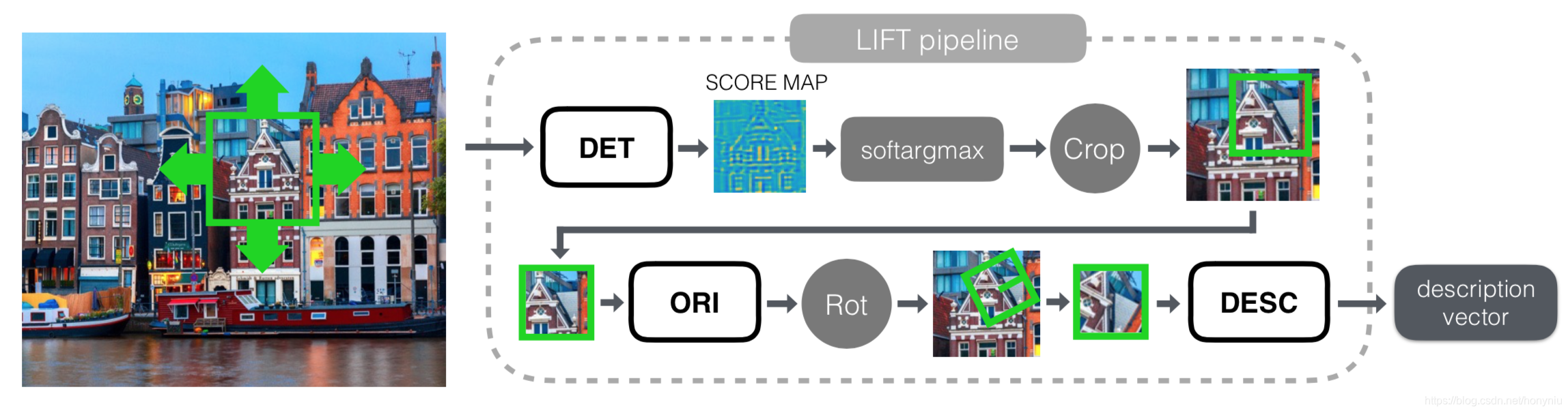
其中包括主要的部分 Detector、Orientation Estimator 和 Descriptor。每个子任务都是单独的 CNN 网络，之前的工作 TILDE、Learn Orientation 和 DeepDesc 已经证明单独任务利用 CNN 网络可以处理的很好，本文则把它们统一到大框架里一起学习，整个网络架构是端对端可导的。

其中为了把这三个任务合并在一起，这里得到 Detector 和 Orientation Estimator 任务的输出结果后，利用 Spatial Transformers 层得到 patch 作为 Descriptor 任务的输入。

其中用 soft argmax 替代传统检测算法 non-local maximum suppression(NMS) 算法。这样做的好处是整个 pipeline 都是可导的，这样可以统一利用反向传导训练，之前没有其他类似的工作，这个是第一次尝试。

网络架构

LIFT 整体的网络架构如下图所示：

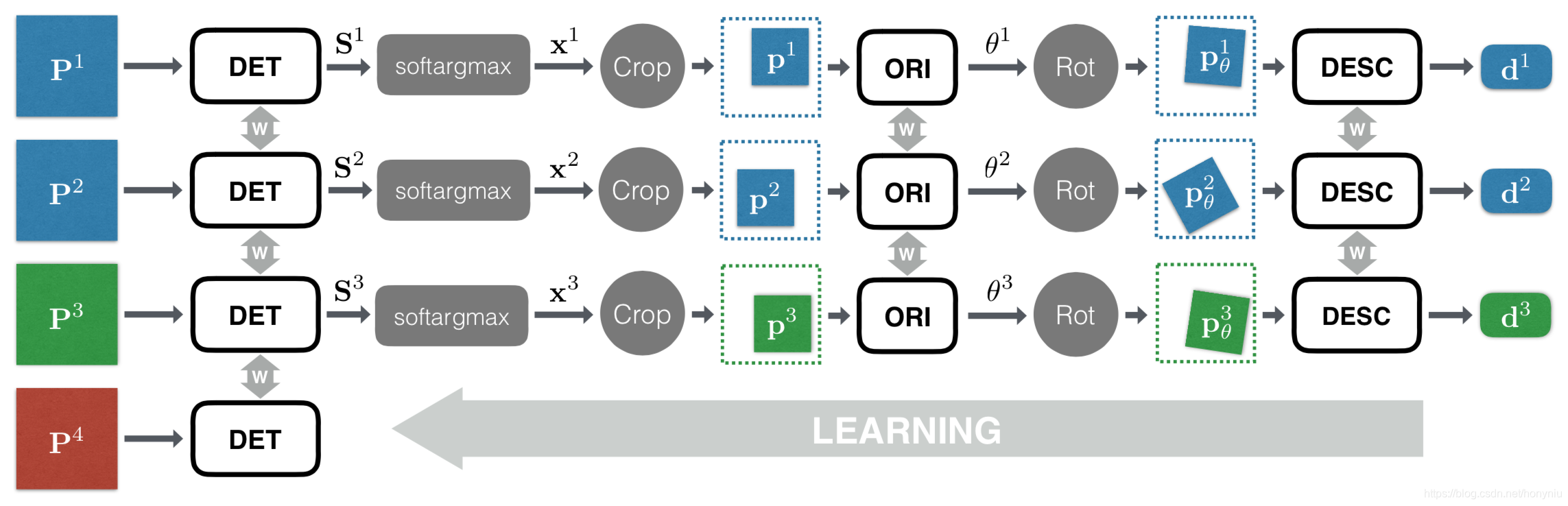
其中网络的输入是 image patches，而不是整张图像，主要是图像中大部分区域并不包含特征点。这些 image patches 是根据特征点提取的，特征点是 SIFT-SfM 构建的，后面会详细讨论。 有个问题是，训练可以这样制造 patches，但是测试时 patches 怎么获得？？？ 而且 image patch 尽可能选择的小，这样保证在给定的这个 scale 的 image patch 上只有一个主要的特征点存在，减少了查找该 image patch 其他特征点时间。 有点奇怪，这还叫特征点 Detector？？？

其中整体网络架构包含四个分支，每个分支都包含 Detector、Orientation Estimator 和 Descriptor 三个不同的 CNN 网络。

在训练过程中，使用 image patches 四元组作为输入。四元组包含两个匹配的 image patches，${\mathbf{P}}^1$ 和 ${\mathbf{P}}^2$（对应同一个 3D 点，在不同的 view 上），第三个 image patch ${\mathbf{P}}^3$ 表示不同的 3D 对应的 patches，第四个 image patch ${\mathbf{P}}^4$ 表示不对应任何 3D 点，上面也不包含特征点。四元组中的四个 image patches 对应网络结构中的四个分支。 但是第四个分支去的其实有问题，有些 patches 在 SfM 中并没有对应 3D 点可能有很多原因，不一定就不包含特征点，这种数据设计是由噪声的？？？？

为了实现端到端的求导，每个分支各个任务的连接关系如下：

1. 输入 image patch $\mathbf{P}$，Detector 输出 score map $\mathbf{S}$；
2. 在 score map $\mathbf{S}$ 上执行 soft argmax 获取特征点位置 $\mathbf{x}$； 如果不存在呢？？？
3. 以特征点位置 $\mathbf{x}$ 为中心，利用 Spatial Transformer 层去 Crop 提取小 patch $\mathbf{p}$ 作为 Orientation Estimator 的输入；
4. Orientation Estimator 估计 $\mathbf{p}$ 的 orientation $\theta$；
5. 然后利用 Spatial Transformer 层根据 $\theta$ 去 rotate $\mathbf{p}$ 得到 ${\mathbf{p}}_{\theta }$；
6. ${\mathbf{p}}_{\theta }$ 输入到 Descriptor 网络得到最终的特征向量 $\mathbf{d}$；

soft argmax 使 argmax 变为可导，将 score map 转换为具体坐标，需要 check 具体公式；

这里提供的 Spatial Transformer 层不具有学习参数，只是为了保持整体可导，操作需要的参数在前面 CNN 中已经求得 $\mathbf{x}$ 和 $\theta$，Spatial Transformer 层只需要根据这两个值对 image patches 进行 Crop 和 Rot 即可。

整个网络作为整体一起从 scratch 开始 train 比较难收敛。所以本文设计了一种针对特定任务学习流程，首先学习 Descriptor 的参数，然后基于学习到的参数学习 Orientation Estimator 的参数，最后根据前两个已经学到的参数去学习 Detector 的参数。从后向前去训练每个部分，这样最后的梯度也可以正确的反向传导。

构建训练数据集

从 1DSfM 提供的 13 个数据集中选择 Piccadilly Circus 和 Roman Forum 两个数据集。然后利用 VisualSFM 进行重建(基于 SIFT 特征点)得到 3D 点。具体重建后每个数据集内容如下：

1. Piccadilly 包含 3384 张图像，$59k$ 个 3D 点，平均每个 3D 点有 6.5 个图像观察到；
2. Roman-Forum 包含 1658 张图像，$51k$ 个 3D 点，平均每个 3D 点有 5.2 个图像观察到；

数据集中的一些图像示例如下：

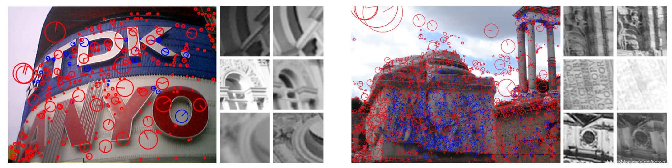
其中左边图像来自 Piccadilly 数据集，右边图像来自 Roman-Forum 数据集。在 SfM 重建过程中保留下来的特征点为蓝色，其他的为红色。

把上面收集到的数据集分为训练集和验证集，如果训练集中某些 3D 在验证集合也被观察到，那就删除验证集合中观察到这些点的 view，同理也删除训练集中观察到验证集中 3D 点的那些 view。 具体怎么划分的感觉还是有点问题？？？

构建正样本匹配的 patch pair 只从 SfM 重建保留下来的特征中选择(这些点鲁棒性强，当做特征点合适)。同时为了提取不包含任何特征点的 patches(上面说的网络结构中第四个分支的输入)，随机采用不包含 SIFT 特征的图像区域，当然那些在 SfM 过程没保留下来的特征点也不能被包含。

根据点的 scale $\sigma$ 值，去在原图上提取灰度的 image patches $\mathbf{P}$。 patches $\mathbf{P}$ 在给定的位置上提取 $24\sigma \times 24\sigma$ 的区域，然后标准化到 $S\times S$，其中 $S=128$。然后小的 patches $\mathbf{p}$ 和 ${\mathbf{p}}_{\theta }$ 作为 Orientation Estimator 和 Descriptor 网络的输入，大小都是 $s\times s$，其中 $s=64$。

这里后面说小 patches 和 SIFT描述符的支持区域大小 $12\sigma$ 对应起来，不太明白？？？

为了防止 overfitting，在 patch 位置上做了随机扰动，范围是 $20\%(4.8\sigma )$。最后利用整个数据集灰度图的均值和标准差归一化输入的 patches。

Descriptor

本文利用 DeepDesc 提供的网络结构去提取 patches 的描述符。在训练 Descriptor 网络的时候，Detector 和 Orientation Estimator 不参与训练。该网络的输入的是 Orientation Estimator 输出 ${\mathbf{p}}_{\theta }$。但是此时前面的网络还没有训练，不能自动生成，这里使用 SfM 得到的特征点的位置和 ori 来生成 ${\mathbf{p}}_{\theta }$，当做 Descriptor 网络的训练数据。

训练 Descriptor 网络，主要是最小化匹配 patch pairs 之间的 Euclidean 距离，最大化非匹配patch pairs 之间的 Euclidean 距离，具体的 loss 公式如下：

$${\mathcal{L}}_{\mathrm{d}\mathrm{e}\mathrm{s}\mathrm{c}}\left({\mathbf{p}}_{\theta }^k,{\mathbf{p}}_{\theta }^l\right)=\{\begin{array}{lc}{\Vert h_{\rho }\left({\mathbf{p}}_{\theta }^k\right)-h_{\rho }\left({\mathbf{p}}_{\theta }^l\right)\Vert }_2& \text{ for positive pairs, and }\\ \max \left(0,C-{\Vert h_{\rho }\left({\mathbf{p}}_{\theta }^k\right)-h_{\rho }\left({\mathbf{p}}_{\theta }^l\right)\Vert }_2\right)& \text{ for negative pairs }\end{array}$$

其中 $\mathbf{d}=h_{\rho }\left({\mathbf{p}}_{\theta }\right)$，$h(.)$ 表示 Descriptor 网络，$\rho$ 表示 CNN 网络参数。

其中 $C=4$ 表示非匹配 patch pair 的最大距离边界（距离更远 loss 不继续增加了）。

在训练 Descriptor 网络使用 hard mining 方法，和上面 DeepDesc 中使用方法一样，在 DeepDesc 中也看出该策略对最终的描述符的性能很重要。基于该策略，总共输入 $K_f$ 个 pairs，然后只取 loss 最高的前 $K_b$ 个 paris 的 loss 进行反向传播，$r=K_f/K_b\ge 1$ 表示 mining ratio。在 DeepDesc 工作中，网络预训练没使用 mining 策略，fine-tune 时候设置 $r=8$。本文使用增量是的 mining 策略，训练开始 $r=1$，然后每 5000 个 batches 后 $r$ 翻倍。这里每个 batch 包括 128 对正样本，128 对负样本。

Orientation Estimator

本文进行 Orientation Estimator 的思路和 Learn Orientation 类似。但该方法需要预先计算好多个 orientation 的描述符向量，然后计算相对于 orientation 的 Jacobian 矩阵。 这里说的 Jacobian 具体含义？？？ 在本文中 Detector 的输入没有直接处理，而是作为整个 pipeline 的一部分，所以预先计算描述符向量是不可能的。

基于上面的考虑，本文采用 Spatial Transformers 去学习 orientation。根据 Detector 网络输出的区域位置可以得到 patch $\mathbf{p}$，然后 Orientation Estimator 估计一个 orientation，公式如下：

$$\theta =g_{\varphi }(\mathbf{p})$$

其中 $g(.)$ 表示 Orientation Estimator 网络，$\varphi$ 表示 CNN 网络参数。

这样给定原始的 image patch $\mathbf{P}$，以及 Detector 网络的输出位置 $\mathbf{x}$，还有第二个 Spatial Transformer 层 $\mathrm{Rot}(.)$ 估计的 $\theta$，这样 Descriptor 网络的输入得到了 ${\mathbf{p}}_{\theta }=\mathrm{Rot}(\mathbf{P},\mathbf{x},\theta )$。

这样在训练 Orientation Estimator 网络的时候，可以最小化相同 3D 点在不同 views 下的特征向量的距离，loss 最终还是落在 Descriptor 网络上。同时在训练时固定前面已经训练好的 Descriptor 的参数，同时 Detector 还是不继续训练，使用 SfM 得到的特征点的位置信息生成。训练 Orientation Estimator 网络 loss 的公式如下：

$${\mathcal{L}}_{\text{ orientation }}\left({\mathbf{P}}^1,{\mathbf{x}}^1,{\mathbf{P}}^2,{\mathbf{x}}^2\right)={\Vert h_{\rho }\left(G\left({\mathbf{P}}^1,{\mathbf{x}}^1\right)\right)-h_{\rho }\left(G\left({\mathbf{P}}^2,{\mathbf{x}}^2\right)\right)\Vert }_2$$

简单来说就是最小化匹配 pairs 特征向量之间的 Euclidean 距离。

其中 $G(\mathbf{P},\mathbf{x})=\mathrm{Rot}\left(\mathbf{P},\mathbf{x},g_{\varphi }(\mathrm{Crop}(\mathbf{P},\mathbf{x}))\right)$，表示前面的 crop 和 rotate 操作。

其中 $\left({\mathbf{P}}^1,{\mathbf{P}}^2\right)$ 表示同一个 3D 点的投影对应的 image patches，${\mathbf{x}}^1$ 和 ${\mathbf{x}}^2$ 分布表示投影位置。

Detector

Detector 网络输入一个 image patch，返回一个 score map。本文的方法和 TILDE 类似，卷积层后面跟着分段线性激活函数，具体如下：

$$\mathbf{S}=f_{\mu }(\mathbf{P})=\sum _n^N{\delta }_n\underset{m}{\max }\left({\mathbf{W}}_{mn}\ast \mathbf{P}+{\mathbf{b}}_{mn}\right)$$

其中 $f_{\mu }(\mathbf{P})$ 表示 Detector 网络， $\mu$ 表示 CNN 网络参数。

其中 ${\delta }_n=\{\begin{array}{lc}+1& \text{ for n is odd, and }\\ -1& \text{ otherwise }\end{array}$

$N$ 和 $M$ 是超参，控制分段线性激活函数的复杂度。

上面公式部分有点不明白

这里和 TILDE 主要的不同是本文使用 score map 中最大值来隐式的表示位置信息，而不是像 TILDE 网络直接去回归 SfM 得到的特征点固定的位置，在实验中发现这样直接回归位置会降低性能。

然后有 score map $\mathbf{S}$，可以得到特征点的位置：

$$\mathbf{x}=\text{ softargmax }(\mathbf{S})$$

其中 softargmax 函数主要计算 score map 的质心，具体公式如下：

$$\mathrm{softargmax}(\mathbf{S})=\frac{{\sum }_{\mathbf{y}}\exp (\beta \mathbf{S}(\mathbf{y}))\mathbf{y}}{{\sum }_{\mathbf{y}}\exp (\beta \mathbf{S}(\mathbf{y}))}$$

其中 $\mathbf{y}$ 是 score map $\mathbf{S}$ 的位置，$\beta =10$ 是控制 softargmax 函数平滑度的超参。softargmax 也可以理解为一个可导的非极大值抑制函数（NMS）。$\mathbf{x}$ 和 image patch $\mathbf{P}$ 输入到第一个 Spatial Transformer 层 $\text{ Crop }(.)$ 函数里面，$\mathbf{p}=\mathrm{Crop}(\mathbf{P},\mathbf{x})$ 可以作为 Orientation Estimator 的输入。

而且之前 Orientation Estimator 网络和 Descriptor 网络都已经训完成，这样就可以固定这两个网络的参数，基于整个 pipeline 来训练。就像上面提到的，输入训练四元组 $\left({\mathbf{P}}_0^1,{\mathbf{P}}^2,{\mathbf{P}}^3,{\mathbf{P}}^4\right)$，最小化 loss 总和，具体如下：

$${\mathcal{L}}_{\text{ detector }}\left({\mathbf{P}}^1,{\mathbf{P}}^2,{\mathbf{P}}^3,{\mathbf{P}}^4\right)=\gamma {\mathcal{L}}_{class}\left({\mathbf{P}}^1,{\mathbf{P}}^2,{\mathbf{P}}^3,{\mathbf{P}}^4\right)+{\mathcal{L}}_{pair}\left({\mathbf{P}}^1,{\mathbf{P}}^2\right)$$

其中 $\gamma$ 是平衡上面两个 loss 的超参。

首先需要对输入的 image patch 进行分类，判断该 patch 上是不是包含一个特征点：

$${\mathcal{L}}_{\mathrm{c}\mathrm{l}\mathrm{a}\mathrm{s}\mathrm{s}}\left({\mathbf{P}}^1,{\mathbf{P}}^2,{\mathbf{P}}^3,{\mathbf{P}}^4\right)=\sum _{i=1}^4{\alpha }_i\max {\left(0,\left(1-\mathrm{softmax}\left(f_{\mu }\left({\mathbf{P}}^i\right)\right)y_i\right)\right)}^2$$

其中 $ \left{ \begin{array} { l } { y _ { i } = - 1 \text { and } \alpha _ { i } = 3 / 6 } & { \text { for i = 4, and } } \ { y _ { i } = + 1 \text { and } \alpha _ { i } = 1 / 6 } & { \text { otherwise } } \end{array} \right.$ 主要是用于正负样本，是不是特征点 patch。这里的分类应该主要是该 patch 是不是包含特征点，是和否，只有两类，但是输入 score map，怎么进行两类的 softmax？？？

然后需要确定特征点位置，这里假设匹配 patch 学习到的位置需要尽可能使根据该位置计算出的描述符直接的距离最近，公式如下：这样其实有可能带来副作用，描述符最近的位置点不一定是正确的匹配点位置？？？
$$\begin{array}{rl}{\mathcal{L}}_{\mathrm{p}\mathrm{a}\mathrm{i}\mathrm{r}}\left({\mathbf{P}}^1,{\mathbf{P}}^2\right)=\Vert & h_{\rho }\left(G\left({\mathbf{P}}^1,\mathrm{softargmax}\left(f_{\mu }\left({\mathbf{P}}^1\right)\right)\right)\right)-h_{\rho }\left(G\left({\mathbf{P}}^2,\mathrm{softargmax}\left(f_{\mu }\left({\mathbf{P}}^2\right)\right)\right)\right)\end{array}$$

这里三个组件一起来促进 Detector 网络的训练，同时设置 Descriptor 网络的 mining ratio 为 $r=8$。

同时文中提到在训练 Descriptor 网络时，已经学习到一些不变性(平移或者说是位置的不变性)，这样对于 Detector 网络来说很难进一步去学习到有用的信息了。为了让 Detector 网络去学习到正确的区域，预训练时限制学习到的位置匹配 patch 必须完全 overlap 在一起，是不是实际输入的位置在 image patch 上就是一样的？？？，后面继续训练时解除限制。

预训练时的 loss 用下面的替换：

$${\tilde{\mathcal{L}}}_{\mathrm{p}\mathrm{a}\mathrm{i}\mathrm{r}}\left({\mathbf{P}}^1,{\mathbf{P}}^2\right)=1-\frac{{\mathbf{p}}^1\cap {\mathbf{p}}^2}{{\mathbf{p}}^1\cup {\mathbf{p}}^2}+\frac{\max \left(0,{\Vert {\mathbf{x}}^1-{\mathbf{x}}^2\Vert }_1-2s\right)}{\sqrt{{\mathbf{p}}^1\cup {\mathbf{p}}^2}}$$

当 ${\tilde{\mathcal{L}}}_{\text{ pair }}=0$ 也就是两个 patch 完全 overlap 在一起。

其中 ${\mathbf{x}}^j=\mathrm{softargmax}\left(f_{\mu }\left({\mathbf{P}}^j\right)\right)$， ${\mathbf{p}}^j=\mathrm{Crop}\left({\mathbf{P}}^j,{\mathbf{x}}^j\right)$，$\Vert \cdot {\Vert }_1$ 是 $l_1\text{ norm }$。

其中 $s=64$ 是 $\mathbf{p}$ 的长和宽。

Pipeline

整体的运行框架如下图所示：

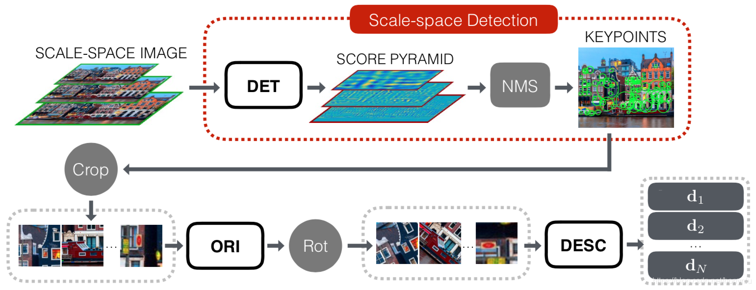
虽然本文方法训练时在 image patches 上进行的，但是测试的输入是整张图像，这里采用在整张图像是进行 sliding window 选取 image patches 的方法。但这样操作，时间花费太大。但幸运的是，Orientation Estimator 和 Descriptor 网络只需要在局部最大值上运行，而不需要在所有的 windows 上运行。这里就把 Detector 网络单独拿出来在整张图像上运行，如上图红框所示，而且是在多个 scale 上运行的，这样把多个 patches 的 score map 合并到原图上，得到了 score pypamid，后面用 NMS（和 SIFT 中使用的一致） 方法代替网络里面的 softargmax 得到最终的 keypoints 的位置。后面的流程就和训练一致了。

实验

数据集和试验构建

三个标准数据集：

1. Strecha 数据集，包含 2 个 scenes 的 19 张 viewpoint 变化的图像。
2. DTU 数据集，包含 60 个 objects 的 60 个序列，包括了 viewpoint 和 illumination，网址如下data。用该数据集评价在不同 viewpoint 下本文方法性能。
3. Webcam 数据集，包含 6 个 scenes 的 710 张 illumination 变化的图像（同一个 viewpoint ）。用该数据集评价在不同 illumination 下本文方法性能。

对于 Strecha 和 DTU 数据集，用于原文作者提供的真值构建匹配关系。每张图像最多使用 1000 个 keypoints，利用 A performance evaluation of local descriptors 提出的评估方法进行评估，主要包含以下指标：

1. Repeatability (Rep.) ：度量特征点的可重复性，表示为一个比例值。主要是评价特征点 Detector 性能，具体指特征点在真值区域被发现的比例。
2. Nearest Neighbor mean Average Precision (NN mAP) ：主要是评价描述符 Descriptor 的可区分度，具体指在不同描述符距离阈值下的 Precision-Recall 曲线的 Area Under Curve (AUC)，使用 NN 匹配策略。
3. Matching Score (M. Score) ：主要是度量整个 pipeline 的性能，具体指真值匹配关系被发现的比例。

效果对比

和 SIFT 对比效果如下图所示：

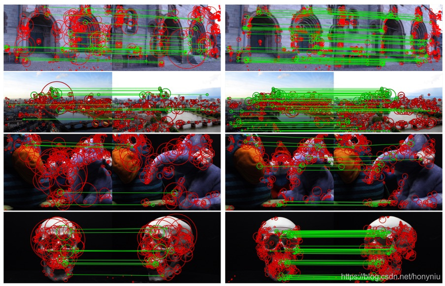
其中左边是 SIFT 结果，右边是本文结果。从上到下测试数据来源分别为Strecha，Webcam，DTU scene 7 和 DTU scene 19 数据集。可以看出本文方法可以得到更多的正确匹配关系。

训练使用的 Piccadilly 数据集，训练集和测试集的区别还是比较大的，但是效果都还不错，说明泛化性能比较强。

整个 pipeline 的量化评估

下图是在三个测试数据集上平均 matching score 对比，具体结果如下图所示：

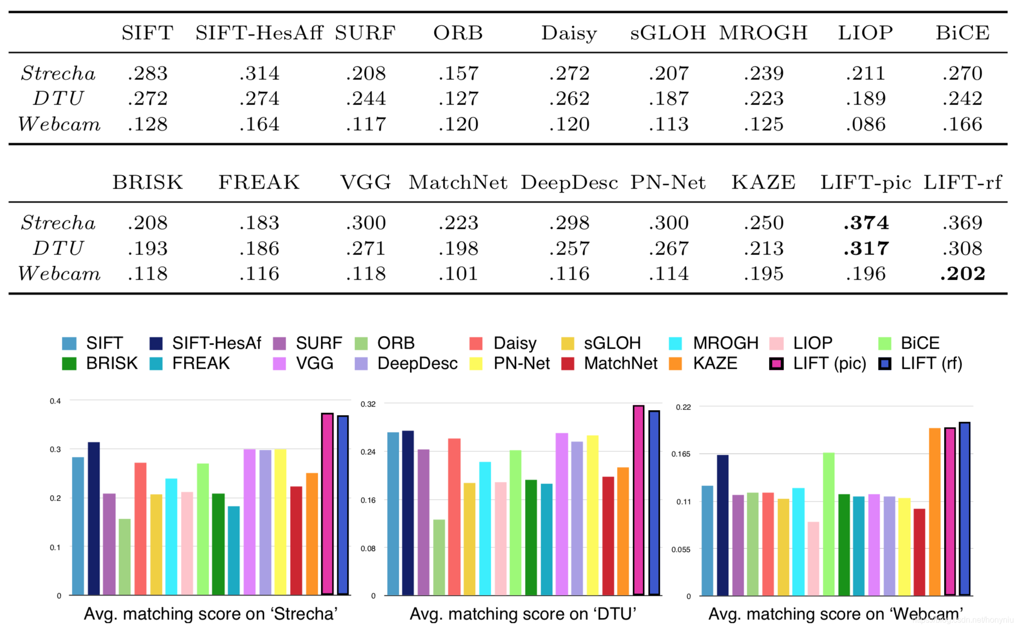
其中 LIFT (pic) 是在 Piccadilly 数据集上训练的，LIFT (rf) 是在 Roman-Forum 数据集上训练的。

同时上面看出 SIFT 效果要好于 VGG，DeepDesc 和 PN-Net 等深度学习方法。

而且对于某些方法单个部分比如 Detector 和 Descriptor 性能可能会好，但在整体 pipeline 评估中性能不一定保持。这也说明整个 pipeline 要放在一起进行学习，像本文方法一样，而且在评估中要考虑对整个 pipeline 的评估。

各部分性能评估

Fine-tuning the Detector

上面讨论 Detector 网络进行预训练和 fine tune 训练，这里对比了这两种性能，具体结果如下图所示：

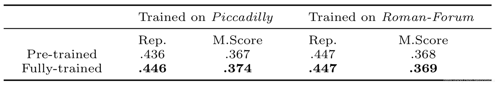
其中是在 Strecha 数据集上进行测试的。看出来只进行预训练性能已经比较好了，fine tune 后性能还是有一些提高的。

而且可以看出来在 Piccadilly 数据集上训练性能比 Roman-Forum 数据集上训练要好一些。主要是因为 Roman-Forum 数据集上没有很多的非特征点区域，也就是说 Detector 训练过程负样本是不足的，在训练过程很容易 over-fitting。

各部分性能

各个部分性能对比如下图所示：

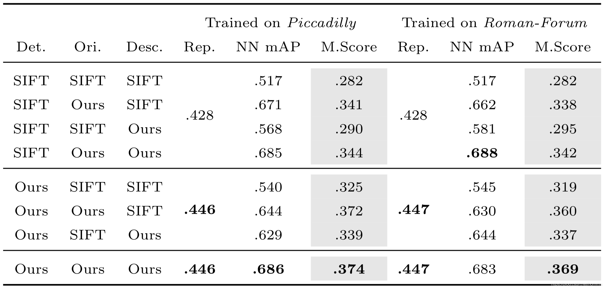
其中是在 Strecha 数据集上进行测试的。

通过上面发现用本文方法替换 SIFT 中的每个部分都会有提高。而且主要是用本文的 Detector 网络替换 SIFT 的检测方法不仅对 Rep 性能有提高，而且对 NN mAP 和 M. Score 都有提高，这说明本文方法不仅可以正确找到特征点位置，而且能找到更利于描述符匹配的位置。同时说明整个 pipeline 一起训练来说是最优的方案。