


14. 隐马尔科夫(HMM,Hidden Markov Model)
14.1 背景
14.1.1 概念回顾
- 机器学习派别
机器学习大致可分两派别:频率派和贝叶斯派的方法。- 频率派
频率派的思想就衍生出了统计学习方法,统计学习方法的重点在于优化,找loss function。频率派的方法可以分成三步:- 定义Model,比如 f ( w ) = w T x + b f(w) = w^Tx+b f(w)=wTx+b;
- 寻找策略strategy,也就是定义Loss function;
- 求解,寻找优化的方法,比如梯度下降(GD),随机梯度下降(SGD),牛顿法,拟牛顿法等等。
- 贝叶斯派
- 贝叶斯派的思想衍生出概率图模型。概率图模型重点研究的是Inferenc问题, 求 一 个 后 验 概 率 分 布 P ( Z ∣ X ) \color{red}求一个后验概率分布P(Z|X) 求一个后验概率分布P(Z∣X),其中 X X X为观测变量, Z Z Z为隐变量。
- 实际上就是一个积分问题,因为贝叶斯框架中的归一化因子需要对整个状态空间进行积分,非常的复杂。代表性的有前面讲到的MCMC,MCMC的提出才是把贝叶斯理论代入到实际的运用中。
- 频率派
- 概率图模型回顾
- 分类
- 概率图模型,如果不考虑时序的关系,大致的分为:有向图的Bayesian Network和无向图的Markov Random Field (Markov Network)。
- 根据分布获得的样本之间都是iid (独立同分布)的。比如Gaussian Mixture Model (GMM),从
P
(
X
∣
θ
)
P(X|\theta)
P(X∣θ)的分布中采出N个样本
{
x
1
,
x
2
,
⋯
,
x
n
}
\{ x_1,x_2,\cdots,x_n \}
{x1,x2,⋯,xn}。N个样本之间都是独立同分布的。也就是对于隐变量
Z
Z
Z,观测变量
X
X
X之间,我们可以假设
P
(
X
∣
Z
)
=
N
(
μ
,
Σ
)
P(X|Z) = \mathcal{N}(\mu,\Sigma)
P(X∣Z)=N(μ,Σ),这样就可以引入我们的先验信息,从而简化
X
X
X的复杂分布。

- 动态模型
对于采出 N N N个样本 { x 1 , x 2 , ⋯ , x n } \{ x_1,x_2,\cdots,x_n \} {x1,x2,⋯,xn},如果引入了时间的信息,也就是 x i x_i xi之间不再iid,我们称之为Dynamic Model。Dynamic Model拓扑结构图如下所示:
- 分类
D y n a m i c M o d e l { 离 散 → H M M 连 续 → { 线 性 → K a l m a n F i l t e r 非 线 性 → P a r t i c l e F i l t e r D y n a m i c M o d e l \left \{ \begin{matrix} 离散\rightarrow\;\;\;\;\;\;\;\;\;\;\;\;\;\;\;\; \;\;\;HMM\;\;\;\;\;\;\;\;\;\;\;\;\;\;\\ 连续\rightarrow \left\{\begin{matrix} 线性\;\;\;\rightarrow Kalman\; Filter\\ 非线性\rightarrow Particle\; Filter \end{matrix}\right. \end{matrix}\right. Dynamic Model⎩⎨⎧离散→HMM连续→{线性→KalmanFilter非线性→ParticleFilter
14.1.2 HMM算法简介
-
相关定义
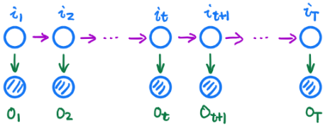
Hidden Markov Model的拓扑结构图如下所示:
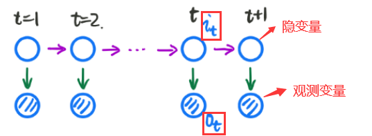
- 拓扑结构图的第一行为 状 态 变 量 i \color{red}状态变量i 状态变量i: I = { i 1 , i 2 , ⋯ , i t , ⋯ } \color{red}I=\{i_1,i_2,\cdots,i_t,\cdots\} I={i1,i2,⋯,it,⋯},每个状态包含 Q = { q 1 , q 2 , ⋯ , q N } \color{red}\mathcal{Q} = \{q_1,q_2,\cdots,q_N\} Q={q1,q2,⋯,qN}。其中 Q \mathcal{Q} Q是状态变量 i i i的 值 域 \color{blue}值域 值域,每个状态变量 i i i可能有 N N N个状态。
- 拓扑结构图的第二行为 观 测 变 量 o \color{red}观测变量o 观测变量o: O = { o 1 , o 2 , ⋯ , o t , ⋯ } \color{red}O=\{o_1,o_2,\cdots,o_t,\cdots\} O={o1,o2,⋯,ot,⋯},每个状态包含 V = { v 1 , v 2 , ⋯ , v M } \color{red}\mathcal{V} = \{v_1,v_2,\cdots,v_M\} V={v1,v2,⋯,vM}。其中 V \mathcal{V} V是观察变量 o o o的 值 域 \color{blue}值域 值域,每个观测变量 o i o_i oi可能有 M M M个状态。
- HMM可以看做一个三元组
λ
=
(
π
,
A
,
B
)
\color{red}\lambda = (\pi, \mathcal{A}, \mathcal{B})
λ=(π,A,B)。其中:
- π \color{red}\pi π:初始概率分布。
- A \color{red}\mathcal{A} A:状态转移矩阵。
- B \color{red}\mathcal{B} B:发射矩阵。
- A = [ a i j ] \color{red}\mathcal{A} = [a_{ij}] A=[aij]表示 状 态 转 移 矩 阵 \color{red}状态转移矩阵 状态转移矩阵, a i j = P ( i ( i + 1 ) = q j ∣ i ( t ) = q i ) \color{red}a_{ij} = P(i_{(i+1)}=q_j|i_{(t)}=q_i) aij=P(i(i+1)=qj∣i(t)=qi)。 A \mathcal{A} A表示为各个状态转移之间的概率。
- B = [ b j ( k ) ] \color{red}\mathcal{B} = [b_j(k)] B=[bj(k)]表示 发 射 矩 阵 \color{red}发射矩阵 发射矩阵, b j ( k ) = P ( o t = V k ∣ i t = q j ) \color{red}b_j(k) = P(o_t = V_k | i_t = q_j) bj(k)=P(ot=Vk∣it=qj)。 B \mathcal{B} B表示为观测变量和隐变量之间的关系。
- 而 π \color{red}\pi π是什么意思呢?假设当 t t t时刻的隐变量 i t i_t it,可能有 { q 1 , q 2 , ⋯ , q N } \color{red}\{ q_1,q_2,\cdots,q_N \} {q1,q2,⋯,qN}个状态,而这些状态出现的概率分别为 { p 1 , p 2 , ⋯ , p N } \color{blue}\{ p_1,p_2,\cdots,p_N \} {p1,p2,⋯,pN}。这就是一个关于 i t i_t it隐变量的离散随机分布。
-
两个假设
这是有关Hidden Markov Model的两个假设:
齐次Markov假设(无后效性) 和 观察独立假设。-
齐次马尔可夫假设:
\textbf{齐次马尔可夫假设:}
齐次马尔可夫假设:
未来与过去无关,只依赖与当前的状态。也就是:
P ( i t + 1 ∣ i t , i t − 1 , ⋯ , i 1 , o t , ⋯ , o 1 ) = P ( i t + 1 ∣ i t ) (14.1.1) P(i_{t+1}|i_{t},i_{t-1},\cdots,i_1,o_t,\cdots,o_1) = P(i_{t+1}|i_t)\tag{14.1.1} P(it+1∣it,it−1,⋯,i1,ot,⋯,o1)=P(it+1∣it)(14.1.1) -
观测独立假设:
\textbf{观测独立假设:}
观测独立假设:
P ( o t ∣ i t , i t − 1 , ⋯ , i 1 , o t , ⋯ , o 1 ) = P ( o t ∣ i t ) (14.1.2) P(o_{t}|i_{t},i_{t-1},\cdots,i_1,o_t,\cdots,o_1) = P(o_{t}|i_t)\tag{14.1.2} P(ot∣it,it−1,⋯,i1,ot,⋯,o1)=P(ot∣it)(14.1.2)
-
齐次马尔可夫假设:
\textbf{齐次马尔可夫假设:}
齐次马尔可夫假设:
-
三个问题
- Evaluation
要求的问题就是 P ( O ∣ λ ) \color{red}P(O|\lambda) P(O∣λ)。也就是前向后向算法,给定一个模型 λ \lambda λ,求出观测变量的概率分布。 - Learning
λ \lambda λ如何求的问题。即: λ M L E = arg max λ P ( O ∣ λ ) \color{red}\lambda_{MLE} = \arg\max_{\lambda}P(O|\lambda) λMLE=argmaxλP(O∣λ)。求解的方法是EM算法和Baum Welch算法。 - Decoding
状态序列为 I I I, I ^ = arg max I P ( I ∣ O , λ ) \color{red}\hat{I} = \arg\max_{I}P(I|O,\lambda) I^=argmaxIP(I∣O,λ)。也就是在在观测变量 O O O和 λ \lambda λ的情况下使隐变量序列 I I I出现的概率最大。而这个问题大致被分为预测和滤波。- 预测问题为: P ( i t + 1 ∣ o 1 , ⋯ , o t ) \color{red}P(i_{t+1}|o_1,\cdots,o_t) P(it+1∣o1,⋯,ot);也就是在已知当前观测变量的情况下预测下一个状态,也就是Viterbi算法。
- 滤波问题为: P ( i t ∣ o 1 , ⋯ , o t ) \color{red}P(i_{t}|o_1,\cdots,o_t) P(it∣o1,⋯,ot);也就是求 t t t时刻的隐变量。
- Evaluation
Hidden Markov Model,可以被我们总结成一个模型 λ = ( π , A , B ) \lambda = (\pi,\mathcal{A},\mathcal{B}) λ=(π,A,B),两个假设,三个问题。而其中关注最多的是Decoding的问题。
14.2 前向算法
14.2.1 概念回顾

图1
- 序列和集合
- I = { i 1 , i 2 , ⋯ , i t , ⋯ , i T } → 状 态 序 列 \color{red}I=\{i_1,i_2,\cdots,i_t,\cdots,i_T\}\rightarrow 状态序列 I={i1,i2,⋯,it,⋯,iT}→状态序列, Q = { q 1 , q 2 , ⋯ , q N } → 状 态 值 集 合 \color{red}\mathcal{Q} = \{q_1,q_2,\cdots,q_N\}\rightarrow 状态值集合 Q={q1,q2,⋯,qN}→状态值集合。
- O = { o 1 , o 2 , ⋯ , o t , ⋯ , o T } → 观 测 序 列 \color{red}O=\{o_1,o_2,\cdots,o_t,\cdots,o_T\}\rightarrow 观测序列 O={o1,o2,⋯,ot,⋯,oT}→观测序列, V = { v 1 , v 2 , ⋯ , v M } → 状 态 值 集 合 \color{red}\mathcal{V} = \{v_1,v_2,\cdots,v_M\}\rightarrow 状态值集合 V={v1,v2,⋯,vM}→状态值集合。
-
λ
=
(
π
,
A
,
B
)
\color{red}\lambda = (\pi, \mathcal{A}, \mathcal{B})
λ=(π,A,B)
- π \color{red}\pi π:初始概率分布。 π = { P ( 1 ) ( 0 ) , P ( 1 ) ( 1 ) , ⋯ , P ( 1 ) ( M ) } \color{red}\pi=\{P_{(1)}(0),P_{(1)}(1),\cdots,P_{(1)}(M)\} π={P(1)(0),P(1)(1),⋯,P(1)(M)}。
- A \color{red}\mathcal{A} A:状态转移矩阵, a i j = P ( i ( i + 1 ) = q j ∣ i ( t ) = q i ) \color{red}a_{ij} = P(i_{(i+1)}=q_j|i_{(t)}=q_i) aij=P(i(i+1)=qj∣i(t)=qi)。
- B \color{red}\mathcal{B} B:发射矩阵, b j ( k ) = P ( o t = V k ∣ i t = q j ) \color{red}b_j(k) = P(o_t = V_k | i_t = q_j) bj(k)=P(ot=Vk∣it=qj)。
- 两个假设
- 齐次马尔可夫假设: \textbf{齐次马尔可夫假设:} 齐次马尔可夫假设: P ( i t + 1 ∣ i t , i t − 1 , ⋯ , i 1 , o t , ⋯ , o 1 ) = P ( i t + 1 ∣ i t ) \color{red}P(i_{t+1}|i_{t},i_{t-1},\cdots,i_1,o_t,\cdots,o_1) = P(i_{t+1}|i_t) P(it+1∣it,it−1,⋯,i1,ot,⋯,o1)=P(it+1∣it)
- 观测独立假设: \textbf{观测独立假设:} 观测独立假设: P ( o t ∣ i t , i t − 1 , ⋯ , i 1 , o t , ⋯ , o 1 ) = P ( o t ∣ i t ) \color{red}P(o_{t}|i_{t},i_{t-1},\cdots,i_1,o_t,\cdots,o_1) = P(o_{t}|i_t) P(ot∣it,it−1,⋯,i1,ot,⋯,o1)=P(ot∣it)
- 三个问题
- Evaluation:Given λ \color{blue}\lambda λ,求 P ( O ∣ λ ) \color{red}P(O|\lambda) P(O∣λ)。(Forward-Backward)
- Learning: λ M L E = arg max λ P ( O ∣ λ ) \color{red}\lambda_{MLE} = \arg\max_{\lambda}P(O|\lambda) λMLE=argmaxλP(O∣λ)。(EM算法和Baum Welch算法)
- Decoding: I ^ = arg max I P ( I ∣ O , λ ) \color{red}\hat{I} = \arg\max_{I}P(I|O,\lambda) I^=argmaxIP(I∣O,λ)。(Viterbi)
本节主要是讲Evaluation中的Forward。
14.2.1 Evaluation-Forward
- 基本方法
- 对于
P
(
O
∣
λ
)
P(O|\lambda)
P(O∣λ)利用概率的基础知识进行化简:
P ( O ∣ λ ) = ∑ I P ( O , I ∣ λ ) = ∑ I P ( O ∣ I , λ ) P ( I ∣ λ ) (14.2.1) P(O|\lambda) = \sum_{I}P(O,I|\lambda) = \sum_{I}P(O|I,\lambda)P(I|\lambda)\tag{14.2.1} P(O∣λ)=I∑P(O,I∣λ)=I∑P(O∣I,λ)P(I∣λ)(14.2.1)
其中:- ∑ I \sum_{I} ∑I表示所有可能出现的隐状态序列;
- ∑ I P ( O ∣ I , λ ) \sum_{I}P(O|I,\lambda) ∑IP(O∣I,λ)表示在某个隐状态下,产生某个观测序列的概率;
-
P
(
I
∣
λ
)
P(I|\lambda)
P(I∣λ)表示某个隐状态出现的概率。那么:
P ( I ∣ λ ) = P ( i 1 , ⋯ , i T ∣ λ ) = P ( i T ∣ i 1 , ⋯ , i T − 1 , λ ) ⋅ P ( i 1 , ⋯ , i T − 1 ∣ λ ) (14.2.2) \begin{array}{ll} P(I|\lambda) & = P(i_1,\cdots,i_T|\lambda) \\ & = P(i_T|i_1,\cdots,i_{T-1},\lambda)\cdot P(i_1,\cdots,i_{T-1}|\lambda) \\\end{array}\tag{14.2.2} P(I∣λ)=P(i1,⋯,iT∣λ)=P(iT∣i1,⋯,iT−1,λ)⋅P(i1,⋯,iT−1∣λ)(14.2.2)
- 根据Hidden Markov Model两个假设
- 齐次马尔可夫假设,可得:
P
(
i
T
∣
i
1
,
⋯
,
i
T
−
1
,
λ
)
=
P
(
i
T
∣
i
T
−
1
)
=
a
i
T
−
1
,
i
T
P(i_T|i_1,\cdots,i_{T-1},\lambda) = P(i_T|i_{T-1}) = a_{i_{T-1},i_T}
P(iT∣i1,⋯,iT−1,λ)=P(iT∣iT−1)=aiT−1,iT。对公式(14.2.2)进行化简可以得到:
P ( i T ∣ i 1 , ⋯ , i T − 1 , λ ) ⋅ P ( i 1 , ⋯ , i T − 1 ∣ λ ) = P ( i T ∣ i T − 1 ) ⋅ P ( i 1 , ⋯ , i T − 1 ∣ λ ) = a i T − 1 , i T ⋅ a i T − 2 , i T − 1 ⋯ a i 1 , i 2 ⋅ π ( a i 1 ) = π ( a i 1 ) ∏ t = 2 T a i t − 1 , i t (14.2.3) \begin{array}{ll} P(i_T|i_1,\cdots,i_{T-1},\lambda)\cdot P(i_1,\cdots,i_{T-1}|\lambda) & = P(i_T|i_{T-1}) \cdot P(i_1,\cdots,i_{T-1}|\lambda) \\ & = a_{i_{T-1},i_T}\cdot a_{i_{T-2},i_{T-1}} \cdots a_{i_1,i_2} \cdot \pi(a_{i_1}) \\ &= \pi(a_{i_1}) \prod_{t=2}^T a_{i_{t-1},i_t}\end{array}\tag{14.2.3} P(iT∣i1,⋯,iT−1,λ)⋅P(i1,⋯,iT−1∣λ)=P(iT∣iT−1)⋅P(i1,⋯,iT−1∣λ)=aiT−1,iT⋅aiT−2,iT−1⋯ai1,i2⋅π(ai1)=π(ai1)∏t=2Tait−1,it(14.2.3) - 观察独立假设,可知:
P ( O ∣ I , λ ) = P ( o 1 , o 2 , ⋯ , o T ∣ I , λ ) = ∏ t = 1 T P ( o t ∣ I , λ ) = ∏ t = 1 T b i t ( o t ) (14.2.4) \begin{array}{ll} P(O|I,\lambda) &= P(o_1,o_2,\cdots,o_T|I,\lambda) \\ &= \prod_{t=1}^T P(o_t|I,\lambda) \\ &= \prod_{t=1}^T b_{i_t}(o_t)\end{array}\tag{14.2.4} P(O∣I,λ)=P(o1,o2,⋯,oT∣I,λ)=∏t=1TP(ot∣I,λ)=∏t=1Tbit(ot)(14.2.4)
- 齐次马尔可夫假设,可得:
P
(
i
T
∣
i
1
,
⋯
,
i
T
−
1
,
λ
)
=
P
(
i
T
∣
i
T
−
1
)
=
a
i
T
−
1
,
i
T
P(i_T|i_1,\cdots,i_{T-1},\lambda) = P(i_T|i_{T-1}) = a_{i_{T-1},i_T}
P(iT∣i1,⋯,iT−1,λ)=P(iT∣iT−1)=aiT−1,iT。对公式(14.2.2)进行化简可以得到:
- 结合公式(14.2.4)和(14.2.3),(14.2.1)可以化简为:
P ( O ∣ λ ) = ∑ I π ( a i 1 ) ∏ t = 2 T a i t − 1 , i t ∏ t = 1 T b i t ( o t ) = ∑ i 1 ⋅ ∑ i 2 ⋯ ∑ i T π ( a i 1 ) ∏ t = 2 T a i t − 1 , i t ∏ t = 1 T b i t ( o t ) (14.2.5) \color{blue}\begin{array}{ll} P(O|\lambda) &= \sum_I \pi(a_{i_1}) \prod_{t=2}^T a_{i_{t-1},i_t} \prod_{t=1}^T b_{i_t}(o_t) \\ &= \sum_{i_1}\cdot \sum_{i_2} \cdots \sum_{i_T} \pi(a_{i_1}) \prod_{t=2}^T a_{i_{t-1},i_t} \prod_{t=1}^T b_{i_t}(o_t)\end{array}\tag{14.2.5} P(O∣λ)=∑Iπ(ai1)∏t=2Tait−1,it∏t=1Tbit(ot)=∑i1⋅∑i2⋯∑iTπ(ai1)∏t=2Tait−1,it∏t=1Tbit(ot)(14.2.5)
公式(14.2.1)共有 T T T个状态,每个状态有 N N N种可能,所以算法复杂度为 O ( N T ) \color{red}\mathcal{O}(N^T) O(NT)。计算太困难了!
- 对于
P
(
O
∣
λ
)
P(O|\lambda)
P(O∣λ)利用概率的基础知识进行化简:
- Forward Algorithm
下图是Hidden Markov Model的拓扑结构图:
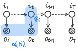
- 思路
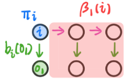
我们记 α t ( i ) = P ( o 1 , ⋯ , o t , i t = q i ∣ λ ) \color{red}\alpha_t(i) = P(o_1,\cdots,o_t,i_t = q_i|\lambda) αt(i)=P(o1,⋯,ot,it=qi∣λ),这个公式表示:在之前所有的观测变量的前提下求出当前时刻的隐变量的概率。那么:
P ( O ∣ λ ) = ∑ i = 1 N P ( O , i T = q i ∣ λ ) = ∑ i = 1 N α T ( i ) (14.2.6) \color{red}P(O|\lambda) = \sum_{i=1}^N P(O, i_T = q_i | \lambda) = \sum_{i=1}^N \alpha_T(i)\tag{14.2.6} P(O∣λ)=i=1∑NP(O,iT=qi∣λ)=i=1∑NαT(i)(14.2.6)
其中, ∑ i = 1 N \sum_{i=1}^N ∑i=1N表示对所有可能出现的隐状态情形求和。通过寻找 α t ( i ) \color{blue}\alpha_t(i) αt(i)和 α t ( i + 1 ) \color{blue}\alpha_t(i+1) αt(i+1)之间的递推关系,就可以得到整个观测序列出现的概率。 - 求解递推关系
α t ( i + 1 ) \alpha_t(i+1) αt(i+1)可以写成:
α t ( i + 1 ) = P ( o 1 , ⋯ , o t , o t + 1 , i t + 1 = q j ∣ λ ) (14.2.7) \color{red}\alpha_t(i+1) = P(o_1,\cdots,o_t,o_{t+1},i_{t+1}=q_j|\lambda)\tag{14.2.7} αt(i+1)=P(o1,⋯,ot,ot+1,it+1=qj∣λ)(14.2.7)
因为 α t ( i ) \alpha_t(i) αt(i)里面有 i t = q j i_{t}=q_j it=qj,因此想办法把 i t i_{t} it给塞进 α t ( i + 1 ) \alpha_t(i+1) αt(i+1)中,即:
α t ( i + 1 ) = P ( o 1 , ⋯ , o t , o t + 1 , i t + 1 = q j ∣ λ ) = ∑ i = 1 N P ( o 1 , ⋯ , o t , o t + 1 , i t = q i , i t + 1 = q j ∣ λ ) = ∑ i = 1 N P ( o t + 1 ∣ o 1 , ⋯ , o t , i t = q i , i t + 1 = q j , λ ) ⋅ P ( o 1 , ⋯ , o t , i t = q i , i t + 1 = q j ∣ λ ) (14.2.7) \begin{array}{ll} \alpha_t(i+1) & = P(o_1,\cdots,o_t,o_{t+1},i_{t+1}=q_j|\lambda) \\ & = \sum_{i=1}^N P(o_1,\cdots,o_t,o_{t+1},i_{t}=q_i,i_{t+1}=q_j|\lambda) \\ & = \sum_{i=1}^N P(o_{t+1}|o_1,\cdots,o_t,i_{t}=q_i,i_{t+1}=q_j,\lambda) \cdot P(o_1,\cdots,o_t,i_{t}=q_i,i_{t+1}=q_j|\lambda)\end{array}\tag{14.2.7} αt(i+1)=P(o1,⋯,ot,ot+1,it+1=qj∣λ)=∑i=1NP(o1,⋯,ot,ot+1,it=qi,it+1=qj∣λ)=∑i=1NP(ot+1∣o1,⋯,ot,it=qi,it+1=qj,λ)⋅P(o1,⋯,ot,it=qi,it+1=qj∣λ)(14.2.7)- 根据观测独立性假设,可得
P
(
o
t
+
1
∣
o
1
,
⋯
,
o
t
,
i
t
=
q
i
,
i
t
+
1
=
q
j
,
λ
)
=
P
(
o
t
+
1
∣
i
t
+
1
=
q
j
)
\color{blue}P(o_{t+1}|o_1,\cdots,o_t,i_{t}=q_i,i_{t+1}=q_j,\lambda) = P(o_{t+1}|i_{t+1}=q_j)
P(ot+1∣o1,⋯,ot,it=qi,it+1=qj,λ)=P(ot+1∣it+1=qj)。所以:
α t ( i + 1 ) = ∑ i = 1 N P ( o t + 1 ∣ o 1 , ⋯ , o t , i t = q i , i t + 1 = q j , λ ) ⋅ P ( o 1 , ⋯ , o t , i t = q i , i t + 1 = q j ∣ λ ) = ∑ i = 1 N P ( o t + 1 ∣ i t + 1 = q j ) ⋅ P ( o 1 , ⋯ , o t , i t = q i , i t + 1 = q j ∣ λ ) (14.2.8) \begin{array}{ll} \alpha_t(i+1) &= \sum_{i=1}^N P(o_{t+1}|o_1,\cdots,o_t,i_{t} = q_i,i_{t+1}=q_j,\lambda) \cdot P(o_1,\cdots,o_t,i_{t} = q_i,i_{t+1}=q_j|\lambda) \\ & = \sum_{i=1}^N P(o_{t+1}|i_{t+1}=q_j)\cdot P(o_1,\cdots,o_t,i_{t}=q_i,i_{t+1}=q_j|\lambda) \end{array}\tag{14.2.8} αt(i+1)=∑i=1NP(ot+1∣o1,⋯,ot,it=qi,it+1=qj,λ)⋅P(o1,⋯,ot,it=qi,it+1=qj∣λ)=∑i=1NP(ot+1∣it+1=qj)⋅P(o1,⋯,ot,it=qi,it+1=qj∣λ)(14.2.8)
看到这个化简后的公式,与 α t ( i ) \alpha_t(i) αt(i)相比,还多了一项 i t + 1 = q j i_{t+1}=q_j it+1=qj,下一步的工作就是消去它。所以:
P ( o 1 , ⋯ , o t , i t = q i , i t + 1 = q j ∣ λ ) = P ( i t + 1 = q j ∣ o 1 , ⋯ , o t , i t = q i , λ ) ⋅ P ( o 1 , ⋯ , o t , i t = q i ∣ λ ) (14.2.9) P(o_1,\cdots,o_t,i_{t}=q_i,i_{t+1}=q_j|\lambda) = P(i_{t+1}=q_j |o_1,\cdots,o_t,i_{t}=q_i,\lambda)\cdot P(o_1,\cdots,o_t,i_{t}=q_i|\lambda)\tag{14.2.9} P(o1,⋯,ot,it=qi,it+1=qj∣λ)=P(it+1=qj∣o1,⋯,ot,it=qi,λ)⋅P(o1,⋯,ot,it=qi∣λ)(14.2.9) - 根据齐次马尔可夫性质,可得
P
(
i
t
+
1
=
q
j
∣
o
1
,
⋯
,
o
t
,
i
t
=
q
i
,
λ
)
=
P
(
i
t
+
1
=
q
j
∣
i
t
=
q
i
)
\color{blue}P(i_{t+1}=q_j |o_1,\cdots,o_t,i_{t}=q_i,\lambda) = P(i_{t+1}=q_j | i_{t}=q_i)
P(it+1=qj∣o1,⋯,ot,it=qi,λ)=P(it+1=qj∣it=qi)。所以:
α t + 1 ( j ) = ∑ i = 1 N P ( o t + 1 ∣ i t + 1 = q j ) ⋅ P ( i t + 1 = q j ∣ i t = q i ) ⋅ P ( o 1 , ⋯ , o t , i t = q i ∣ λ ) = ∑ i = 1 N b j ( o t + 1 ) ⋅ a i j ⋅ α t ( i ) (14.2.10) \begin{array}{ll} \alpha_{t+1}(j) & = \sum_{i=1}^N P(o_{t+1}|i_{t+1}=q_j)\cdot P(i_{t+1}=q_j | i_{t}=q_i) \cdot P(o_1,\cdots,o_t,i_{t}=q_i|\lambda) \\ & = \sum_{i=1}^N b_j(o_{t+1})\cdot a_{ij} \cdot \alpha_t(i) \end{array}\tag{14.2.10} αt+1(j)=∑i=1NP(ot+1∣it+1=qj)⋅P(it+1=qj∣it=qi)⋅P(o1,⋯,ot,it=qi∣λ)=∑i=1Nbj(ot+1)⋅aij⋅αt(i)(14.2.10) - 经过上述的推导,我们就成功的得到了
α
t
+
1
(
j
)
\alpha_{t+1}(j)
αt+1(j)和
α
t
(
i
)
\alpha_t(i)
αt(i)之间的关系:
α t + 1 ( j ) = ∑ i = 1 N b j ( o t + 1 ) ⋅ a i j ⋅ α t ( i ) (14.2.11) \color{red}\alpha_{t+1}(j)= \sum_{i=1}^N b_j(o_{t+1})\cdot a_{ij} \cdot \alpha_t(i)\tag{14.2.11} αt+1(j)=i=1∑Nbj(ot+1)⋅aij⋅αt(i)(14.2.11)
通过这个递推关系,就可以遍历整个Markov Model了。这个公式是什么意思呢?它可以表达为,所有可能出现的隐变量状态乘以转移到状态 j j j的概率,乘以根据隐变量 i t + 1 i_{t+1} it+1观察到 o t + 1 o_{t+1} ot+1的概率,乘上根据上一个隐状态观察到的观察变量的序列的概率。
- 根据观测独立性假设,可得
P
(
o
t
+
1
∣
o
1
,
⋯
,
o
t
,
i
t
=
q
i
,
i
t
+
1
=
q
j
,
λ
)
=
P
(
o
t
+
1
∣
i
t
+
1
=
q
j
)
\color{blue}P(o_{t+1}|o_1,\cdots,o_t,i_{t}=q_i,i_{t+1}=q_j,\lambda) = P(o_{t+1}|i_{t+1}=q_j)
P(ot+1∣o1,⋯,ot,it=qi,it+1=qj,λ)=P(ot+1∣it+1=qj)。所以:
- 思路
- 总结
令 α t ( i ) = P ( o 1 , ⋯ , o t , i t = q i ∣ λ ) P ( O ∣ λ ) = ∑ i = 1 N P ( O , i t = q i ∣ λ ) = ∑ i = 1 N α T ( i ) α t + 1 ( j ) = ∑ i = 1 N b j ( o t + 1 ) ⋅ a i j ⋅ α t ( i ) \color{red}令\alpha_t(i) = P(o_1,\cdots,o_t,i_t = q_i|\lambda)\\ P(O|\lambda) = \sum_{i=1}^N P(O, i_t = q_i | \lambda) = \sum_{i=1}^N \alpha_T(i)\\ \alpha_{t+1}(j)= \sum_{i=1}^N b_j(o_{t+1})\cdot a_{ij} \cdot \alpha_t(i) 令αt(i)=P(o1,⋯,ot,it=qi∣λ)P(O∣λ)=i=1∑NP(O,it=qi∣λ)=i=1∑NαT(i)αt+1(j)=i=1∑Nbj(ot+1)⋅aij⋅αt(i)
用一个图来进行表示: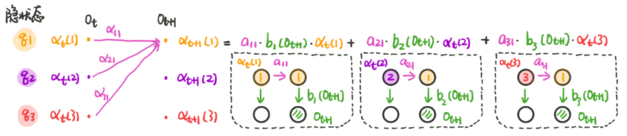
假设有隐状态的状态空间数为 N N N,序列的长度为 T T T,那么总的时间复杂度为 O ( T N 2 ) \color{red}\mathcal{O}(TN^2) O(TN2)。
14.3 后向算法
后向概率的推导实际上比前向概率的理解要难,前向算法是一个联合概率,而后向算法则是一个条件概率,所以后向的概率实际上比前向难求很多。
-
基本思路
下图是Hidden Markov Model的拓扑结构图:
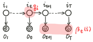
定义:
β t ( i ) = P ( o t + 1 , ⋯ , o T ∣ i t = q i , λ ) (14.3.1) \color{red}\beta _{t}(i)=P(o_{t+1},\cdots ,o_{T}|i_{t}=q_{i},\lambda )\tag{14.3.1} βt(i)=P(ot+1,⋯,oT∣it=qi,λ)(14.3.1)
则 β 1 ( t ) = P ( o 2 , ⋯ , o T ∣ i 1 = q i , λ ) \color{blue}\beta_1(t)= P(o_{2},\cdots,o_T|i_1 = q_i,\lambda) β1(t)=P(o2,⋯,oT∣i1=qi,λ)。计算目标 P ( O ∣ λ ) \color{blue}P(O|\lambda) P(O∣λ)可以表示为::
P ( O ∣ λ ) = P ( o 1 , ⋯ , o T ∣ λ ) = ∑ i = 1 N P ( o 1 , ⋯ , o T , i 1 = q i ∣ λ ) = ∑ i = 1 N P ( o 1 , ⋯ , o T ∣ i 1 = q i , λ ) P ( i 1 = q i ∣ λ ) ⏟ π i = ∑ i = 1 N P ( o 1 ∣ o 2 , ⋯ , o T , i 1 = q i , λ ) P ( o 2 , ⋯ , o T ∣ i 1 = q i , λ ) ⏟ β 1 ( i ) π i = ∑ i = 1 N P ( o 1 ∣ i 1 = q i , λ ) β 1 ( i ) π i = ∑ i = 1 N b i ( o 1 ) β 1 ( i ) π i (14.3.2) \begin{array}{ll}P(O|\lambda )&=P(o_{1},\cdots ,o_{T}|\lambda )\\ &=\sum_{i=1}^{N}P(o_{1},\cdots ,o_{T},i_{1}=q_{i}|\lambda )\\ &=\sum_{i=1}^{N}P(o_{1},\cdots ,o_{T}|i_{1}=q_{i},\lambda )\underset{\pi _{i}}{\underbrace{P(i_{1}=q_{i}|\lambda )}}\\ &=\sum_{i=1}^{N}P(o_{1}|o_{2},\cdots ,o_{T},i_{1}=q_{i},\lambda )\underset{\beta _{1}(i)}{\underbrace{P(o_{2},\cdots ,o_{T}|i_{1}=q_{i},\lambda )}}\pi _{i}\\ &=\sum_{i=1}^{N}P(o_{1}|i_{1}=q_{i},\lambda )\beta _{1}(i)\pi _{i}\\ &=\sum_{i=1}^{N}b_{i}(o_{1})\beta _{1}(i)\pi _{i}\end{array}\tag{14.3.2} P(O∣λ)=P(o1,⋯,oT∣λ)=∑i=1NP(o1,⋯,oT,i1=qi∣λ)=∑i=1NP(o1,⋯,oT∣i1=qi,λ)πi P(i1=qi∣λ)=∑i=1NP(o1∣o2,⋯,oT,i1=qi,λ)β1(i) P(o2,⋯,oT∣i1=qi,λ)πi=∑i=1NP(o1∣i1=qi,λ)β1(i)πi=∑i=1Nbi(o1)β1(i)πi(14.3.2)
现在已成功的找到 P ( O ∣ λ ) 和 第 一 个 状 态 之 间 的 关 系 \color{red}P(O|\lambda)和第一个状态之间的关系 P(O∣λ)和第一个状态之间的关系。其中:- π i \pi_i πi为某个状态的初始状态的概率;
- b i ( o 1 ) b_i(o_1) bi(o1)表示为第 i i i个隐变量产生第1个观测变量的概率;
-
β
1
(
i
)
\beta_1(i)
β1(i)表示为第一个观测状态确定以后生成后面观测状态序列的概率。结构图如下所示:
-
求解递推关系
因此如果我们能找到 β t ( i ) \color{blue}\beta _{t}(i) βt(i)到 β t + 1 ( j ) \color{blue}\beta _{t+1}(j) βt+1(j)的递推式,就可以由通过递推得到 β 1 ( i ) \color{blue}\beta _{1}(i) β1(i),从而计算 P ( O ∣ λ ) P(O|\lambda ) P(O∣λ),则递推公式是:
β t ( i ) = P ( o t + 1 , ⋯ , o T ∣ i t = q i , λ ) = ∑ j = 1 N P ( o t + 1 , ⋯ , o T , i t + 1 = q j ∣ i t = q i , λ ) = ∑ j = 1 N P ( o t + 1 , ⋯ , o T ∣ i t + 1 = q j , i t = q i , λ ) P ( i t + 1 = q j ∣ i t = q i , λ ) = ∑ j = 1 N P ( o t + 1 , ⋯ , o T ∣ i t + 1 = q j , λ ) a i j = ∑ j = 1 N P ( o t + 1 ∣ o t + 2 , ⋯ , o T , i t + 1 = q j , λ ) P ( o t + 2 , ⋯ , o T ∣ i t + 1 = q j , λ ) a i j ( 从 这 一 步 到 下 一 步 满 足 : A ⊥ C ∣ B ⇔ 若 B 被 观 测 , 则 路 径 被 阻 塞 。 ) = ∑ j = 1 N P ( o t + 1 ∣ i t + 1 = q j , λ ) β t + 1 ( j ) a i j = ∑ j = 1 N b j ( o t + 1 ) a i j β t + 1 ( j ) (14.3.3) \begin{array}{ll}\beta _{t}(i)&=P(o_{t+1},\cdots ,o_{T}|i_{t}=q_{i},\lambda )\\ &=\sum_{j=1}^{N}P(o_{t+1},\cdots ,o_{T},i_{t+1}=q_{j}|i_{t}=q_{i},\lambda )\\ &=\sum_{j=1}^{N}{\color{Red}{P(o_{t+1},\cdots ,o_{T}|i_{t+1}=q_{j},i_{t}=q_{i},\lambda)}}{\color{Blue}{P(i_{t+1}=q_{j}|i_{t}=q_{i},\lambda )}}\\ &=\sum_{j=1}^{N}{\color{Red}{P(o_{t+1},\cdots ,o_{T}|i_{t+1}=q_{j},\lambda)}}{\color{Blue}{a_{ij}}}\\ &=\sum_{j=1}^{N}{\color{Orange}{P(o_{t+1}|o_{t+2},\cdots ,o_{T},i_{t+1}=q_{j},\lambda)}}{\color{Orchid}{P(o_{t+2},\cdots ,o_{T}|i_{t+1}=q_{j},\lambda)}}{\color{Blue}{a_{ij}}}\\ & (从这一步到下一步满足:A\perp C|B\Leftrightarrow 若B被观测,则路径被阻塞。)\\ &=\sum_{j=1}^{N}{\color{Orange}{P(o_{t+1}|i_{t+1}=q_{j},\lambda)}}{\color{Orchid}{\beta _{t+1}(j)}}{\color{Blue}{a_{ij}}}\\ &=\sum_{j=1}^{N}{\color{Orange}{b_{j}(o_{t+1})}}{\color{Blue}{a_{ij}}}{\color{Orchid}{\beta _{t+1}(j)}}\end{array}\tag{14.3.3} βt(i)=P(ot+1,⋯,oT∣it=qi,λ)=∑j=1NP(ot+1,⋯,oT,it+1=qj∣it=qi,λ)=∑j=1NP(ot+1,⋯,oT∣it+1=qj,it=qi,λ)P(it+1=qj∣it=qi,λ)=∑j=1NP(ot+1,⋯,oT∣it+1=qj,λ)aij=∑j=1NP(ot+1∣ot+2,⋯,oT,it+1=qj,λ)P(ot+2,⋯,oT∣it+1=qj,λ)aij(从这一步到下一步满足:A⊥C∣B⇔若B被观测,则路径被阻塞。)=∑j=1NP(ot+1∣it+1=qj,λ)βt+1(j)aij=∑j=1Nbj(ot+1)aijβt+1(j)(14.3.3)
其中第五行到第六行的推导 P ( o t + 1 , ⋯ , o T ∣ i t + 1 = q j , i t = q i ) = P ( o t + 1 , ⋯ , o T ∣ i t + 1 = q j ) \color{blue}P(o_{t+1},\cdots,o_T |i_{t+1} = q_j, i_t = q_i) = P(o_{t+1},\cdots,o_T |i_{t+1} = q_j) P(ot+1,⋯,oT∣it+1=qj,it=qi)=P(ot+1,⋯,oT∣it+1=qj)使用的马尔可夫链的性质,每一个状态都是后面状态的充分统计量,与之前的状态无关。
-
总结
定 义 : β t ( i ) = P ( o t + 1 , ⋯ , o T ∣ i t = q i , λ ) P ( O ∣ λ ) = ∑ i = 1 N b i ( o 1 ) β 1 ( i ) π i β t ( i ) = ∑ j = 1 N b j ( o t + 1 ) a i j β t + 1 ( j ) (14.3.4) \color{red}定义:\beta _{t}(i)=P(o_{t+1},\cdots ,o_{T}|i_{t}=q_{i},\lambda )\\ P(O|\lambda )=\sum_{i=1}^{N}b_{i}(o_{1})\beta _{1}(i)\pi _{i}\\ \beta _{t}(i)=\sum_{j=1}^{N}{\color{Orange}{b_{j}(o_{t+1})}}{\color{Blue}{a_{ij}}}{\color{Orchid}{\beta _{t+1}(j)}}\tag{14.3.4} 定义:βt(i)=P(ot+1,⋯,oT∣it=qi,λ)P(O∣λ)=i=1∑Nbi(o1)β1(i)πiβt(i)=j=1∑Nbj(ot+1)aijβt+1(j)(14.3.4)
通过这样的迭代从后往前推,我们就可以得到 β i ( 1 ) \beta_i(1) βi(1)的概率,从而推断出 P ( O ∣ λ ) P(O|\lambda) P(O∣λ)。整体的推断流程图如下图所示:

这就是后向算法,其复杂度也为 O ( T N 2 ) \color{red}O(TN^{2}) O(TN2)。
14.4 Beco Decoding算法(Learning)
14.4.1 问题简化
- 上两节讲的是HMM的Evaluating部分,接下来讲HMM的Learning部分。即目标是:
在
已
知
观
测
数
据
的
情
况
下
求
参
数
λ
\color{blue}在已知观测数据的情况下求参数\lambda
在已知观测数据的情况下求参数λ:
λ M L E = arg max λ P ( O ∣ λ ) (14.4.1) \lambda_{MLE} = \arg\max_{\lambda} P(O|\lambda)\tag{14.4.1} λMLE=argλmaxP(O∣λ)(14.4.1)
因为:
P ( O ∣ λ ) = ∑ I P ( O , I ∣ λ ) = ∑ i 1 ⋯ ∑ i T π i 1 ∏ t = 2 T a i t − 1 , i t ∏ t = 1 T b i 1 ( o t ) (14.4.2) P(O|\lambda) = \sum_I P(O,I|\lambda) = \sum_{i_1}\cdots\sum_{i_T} \pi_{i_1} \prod_{t=2}^T a_{i_{t-1},i_{t}} \prod_{t=1}^T b_{i_1}(o_t)\tag{14.4.2} P(O∣λ)=I∑P(O,I∣λ)=i1∑⋯iT∑πi1t=2∏Tait−1,itt=1∏Tbi1(ot)(14.4.2)
对这个方程的 λ \lambda λ求偏导,实在是太难算了。 - 问题简化
所以考虑使用EM算法。先来回顾一下EM算法:
θ ( t + 1 ) = arg max θ ∫ z log P ( X , Z ∣ θ ) ⋅ P ( Z ∣ X , θ ( t ) ) d Z (14.4.3) \theta^{(t+1)} = \arg\max_\theta \int_z \log P(X,Z|\theta)\cdot P(Z|X,\theta^{(t)}) dZ\tag{14.4.3} θ(t+1)=argθmax∫zlogP(X,Z∣θ)⋅P(Z∣X,θ(t))dZ(14.4.3)
其中:- X → O X\rightarrow O X→O为观测变量;
- Z → I Z\rightarrow I Z→I为隐变量,其中 I I I为离散变量;
-
θ
→
λ
\theta \rightarrow \lambda
θ→λ为参数。
那么,可以将公式(14.4.3)改写为:
λ ( t + 1 ) = arg max λ ∑ I log P ( O , I ∣ λ ) ⋅ P ( I ∣ O , λ ( t ) ) (14.4.4) \lambda^{(t+1)} = \arg\max_\lambda \sum_I \log P(O,I|\lambda)\cdot P(I|O,\lambda^{(t)})\tag{14.4.4} λ(t+1)=argλmaxI∑logP(O,I∣λ)⋅P(I∣O,λ(t))(14.4.4)
每次迭代 λ ( t + 1 ) \lambda^{(t+1)} λ(t+1), λ ( t ) \lambda^{(t)} λ(t)是一个常数,即:
P ( I ∣ O , λ ( t ) ) = P ( I , O ∣ λ ( t ) ) P ( O ∣ λ ( t ) ) (14.4.5) P(I|O,\lambda^{(t)}) = \frac{P(I,O|\lambda^{(t)})}{P(O|\lambda^{(t)})}\tag{14.4.5} P(I∣O,λ(t))=P(O∣λ(t))P(I,O∣λ(t))(14.4.5)
并且 P ( O ∣ λ ( t ) ) P(O|\lambda^{(t)}) P(O∣λ(t))中 λ ( t ) \lambda^{(t)} λ(t)是常数,所以这项是个定量,与 λ \lambda λ无关,所以 P ( I , O ∣ λ ( t ) ) P ( O ∣ λ ( t ) ) ∝ P ( I , O ∣ λ ( t ) ) \color{red}\frac{P(I,O|\lambda^{(t)})}{P(O|\lambda^{(t)})} \propto P(I,O|\lambda^{(t)}) P(O∣λ(t))P(I,O∣λ(t))∝P(I,O∣λ(t))。所以等式(14.4.4)改写为:
λ ( t + 1 ) = arg max λ ∑ I log P ( O , I ∣ λ ) ⋅ P ( I , O ∣ λ ( t ) ) (14.4.6) \color{red}\lambda^{(t+1)} = \arg\max_\lambda \sum_I \log P(O,I|\lambda)\cdot P(I,O|\lambda^{(t)})\tag{14.4.6} λ(t+1)=argλmaxI∑logP(O,I∣λ)⋅P(I,O∣λ(t))(14.4.6)
其中 λ ( t ) = ( π ( t ) , A ( t ) , B ( t ) ) \color{blue}\lambda^{(t)} = (\pi^{(t)}, \mathcal{A}^{(t)}, \mathcal{B}^{(t)}) λ(t)=(π(t),A(t),B(t)),而 λ ( t + 1 ) = ( π ( t + 1 ) , A ( t + 1 ) , B ( t + 1 ) ) \color{blue}\lambda^{(t+1)} = (\pi^{(t+1)}, \mathcal{A}^{(t+1)}, \mathcal{B}^{(t+1)}) λ(t+1)=(π(t+1),A(t+1),B(t+1))。这样做有什么目的呢?可以把 log P ( O , I ∣ λ ) \log P(O,I|\lambda) logP(O,I∣λ)和 P ( I , O ∣ λ ( t ) ) P(I,O|\lambda^{(t)}) P(I,O∣λ(t))变成一种形式。
- 公式优化
对于公式(14.4.6),定义:
Q ( λ , λ ( t ) ) = ∑ I log P ( O , I ∣ λ ) ⋅ P ( O , I ∣ λ ( t ) ) (14.4.7) Q(\lambda,\lambda^{(t)}) = \sum_I \log P(O,I|\lambda)\cdot P(O,I|\lambda^{(t)})\tag{14.4.7} Q(λ,λ(t))=I∑logP(O,I∣λ)⋅P(O,I∣λ(t))(14.4.7)
因为公式(14.4.2)化简可知: P ( O , I ∣ λ ) = π i 1 ∏ t = 2 T a i t − 1 , i t ∏ t = 1 T b i 1 ( o t ) P(O,I|\lambda) = \pi_{i_1} \prod_{t=2}^T a_{i_{t-1},i_{t}} \prod_{t=1}^T b_{i_1}(o_t) P(O,I∣λ)=πi1∏t=2Tait−1,it∏t=1Tbi1(ot)。所以:
Q ( λ , λ ( t ) ) = ∑ I [ ( log π i 1 + ∑ t = 2 T log a i t − 1 , i t + ∑ t = 1 T log b i t ( o t ) ) ⋅ P ( O , I ∣ λ ( t ) ) ] (14.4.8) \color{red}Q(\lambda,\lambda^{(t)}) = \sum_I \left[ \left( \log \pi_{i_1} + \sum_{t=2}^T \log a_{i_{t-1},i_t} + \sum_{t=1}^T \log b_{i_t}(o_t) \right)\cdot P(O,I|\lambda^{(t)}) \right]\tag{14.4.8} Q(λ,λ(t))=I∑[(logπi1+t=2∑Tlogait−1,it+t=1∑Tlogbit(ot))⋅P(O,I∣λ(t))](14.4.8)
14.4.2 求解最优值
- 以
π
(
t
+
1
)
\pi^{(t+1)}
π(t+1)为例,在公式
Q
(
λ
,
λ
(
t
)
)
Q(\lambda,\lambda^{(t)})
Q(λ,λ(t))中,
∑
t
=
2
T
log
a
i
t
−
1
,
i
t
\color{blue}\sum_{t=2}^T \log a_{i_{t-1},i_t}
∑t=2Tlogait−1,it与
∑
t
=
1
T
log
b
i
t
(
o
t
)
\color{blue}\sum_{t=1}^T \log b_{i_t}(o_t)
∑t=1Tlogbit(ot)与
π
\color{blue}\pi
π无关,所以,
π ( t + 1 ) = arg max π Q ( λ , λ ( t ) ) = arg max π ∑ I [ log π i 1 ⋅ P ( O , I ∣ λ ( t ) ) ] = arg max π ∑ i 1 ⋯ ∑ i T [ log π i 1 ⋅ P ( O , i 1 , ⋯ , i T ∣ λ ( t ) ) ] (14.4.9) \begin{array}{ll} \pi^{(t+1)} &= \arg\max_{\pi} Q(\lambda,\lambda^{(t)}) \\ &= \arg\max_{\pi} \sum_I [\log \pi_{i_1} \cdot P(O,I|\lambda^{(t)})] \\ &= \arg\max_{\pi} \sum_{i_1}\cdots \sum_{i_T}[\log \pi_{i_1} \cdot P(O,i_1,\cdots,i_T|\lambda^{(t)})] \end{array}\tag{14.4.9} π(t+1)=argmaxπQ(λ,λ(t))=argmaxπ∑I[logπi1⋅P(O,I∣λ(t))]=argmaxπ∑i1⋯∑iT[logπi1⋅P(O,i1,⋯,iT∣λ(t))](14.4.9)
观察 { i 2 , ⋯ , i T } \{i_2,\cdots,i_T\} {i2,⋯,iT}可知, 联 合 概 率 分 布 求 和 可 以 得 到 边 缘 概 率 \color{blue}联合概率分布求和可以得到边缘概率 联合概率分布求和可以得到边缘概率。所以:
π ( t + 1 ) = arg max π ∑ i 1 [ log π i 1 ⋅ P ( O , i 1 ∣ λ ( t ) ) ] = arg max π ∑ i = 1 N [ log π i ⋅ P ( O , i 1 = q i ∣ λ ( t ) ) ] (14.4.10) \begin{array}{ll} \pi^{(t+1)} &= \arg\max_{\pi} \sum_{i_1} [\log \pi_{i_1} \cdot P(O,i_1|\lambda^{(t)})] \\ &= \arg\max_{\pi} \sum_{i=1}^N [\log \pi_{i} \cdot P(O,i_1=q_i|\lambda^{(t)})] \qquad \end{array}\tag{14.4.10} π(t+1)=argmaxπ∑i1[logπi1⋅P(O,i1∣λ(t))]=argmaxπ∑i=1N[logπi⋅P(O,i1=qi∣λ(t))](14.4.10)
优化问题可以描述为:
{ π ( t + 1 ) = arg max π ∑ i = 1 N [ log π i ⋅ P ( O , i 1 = q i ∣ λ ( t ) ) ] s . t . ∑ i = 1 N π i = 1 (14.4.11) \color{red}\{\begin{array}{ll} \pi^{(t+1)} = \underset{\pi}{\arg\max} \sum_{i=1}^N [\log \pi_{i} \cdot P(O,i_1=q_i|\lambda^{(t)})] \\ s.t. \ \sum_{i=1}^N \pi_i = 1\end{array}\tag{14.4.11} {π(t+1)=πargmax∑i=1N[logπi⋅P(O,i1=qi∣λ(t))]s.t. ∑i=1Nπi=1(14.4.11) - 拉格朗日乘子法求解
根据拉格朗日乘子法,我们可以将损失函数写完:
L ( π , η ) = ∑ i = 1 N log π i ⋅ P ( O , i 1 = q i ∣ λ ( t ) ) + η ( ∑ i = 1 N π i − 1 ) (14.4.12) \mathcal{L}(\pi,\eta) = \sum_{i=1}^N \log \pi_{i} \cdot P(O,i_1=q_i|\lambda^{(t)}) + \eta(\sum_{i=1}^N \pi_i - 1)\tag{14.4.12} L(π,η)=i=1∑Nlogπi⋅P(O,i1=qi∣λ(t))+η(i=1∑Nπi−1)(14.4.12)
使似然函数最大化,则是对损失函数 L ( π , η ) \mathcal{L}(\pi,\eta) L(π,η)求偏导,则为:
L π i = 1 π i P ( O , i 1 = q i ∣ λ ( t ) ) + η = 0 P ( O , i 1 = q i ∣ λ ( t ) ) + π i η = 0 (14.4.13) \begin{array}{ll}& \frac{\mathcal{L}}{\pi_i} = \frac{1}{\pi_i} P(O,i_1=q_i|\lambda^{(t)}) + \eta = 0 \\ & P(O,i_1=q_i|\lambda^{(t)}) + \pi_i\eta = 0\end{array}\tag{14.4.13} πiL=πi1P(O,i1=qi∣λ(t))+η=0P(O,i1=qi∣λ(t))+πiη=0(14.4.13)
又因为 ∑ i = 1 N π i = 1 \sum_{i=1}^N \pi_i = 1 ∑i=1Nπi=1,所以将公式(14.4.13)进行求和,可以得到:
∑ i = 1 N [ P ( O , i 1 = q i ∣ λ ( t ) ) + π i η ] = 0 ⇒ P ( O ∣ λ ( t ) ) + η = 0 (14.4.14) \sum_{i=1}^N [P(O,i_1=q_i|\lambda^{(t)}) + \pi_i\eta] = 0 \Rightarrow P(O|\lambda^{(t)}) + \eta = 0\tag{14.4.14} i=1∑N[P(O,i1=qi∣λ(t))+πiη]=0⇒P(O∣λ(t))+η=0(14.4.14)
所以,我们解得 η = − P ( O ∣ λ ( t ) ) \color{red}\eta = -P(O|\lambda^{(t)}) η=−P(O∣λ(t)),从而推出:
π i ( t + 1 ) = P ( O , i 1 = q i ∣ λ ( t ) ) P ( O ∣ λ ( t ) ) (14.4.15) \color{red}\pi_i^{(t+1)} = \frac{P(O,i_1=q_i|\lambda^{(t)})}{P(O|\lambda^{(t)})}\tag{14.4.15} πi(t+1)=P(O∣λ(t))P(O,i1=qi∣λ(t))(14.4.15)
进而,我们就可以推导出 π ( t + 1 ) = ( π 1 ( t + 1 ) , π 2 ( t + 1 ) , ⋯ , π N ( t + 1 ) ) \color{blue}\pi^{(t+1)} = (\pi_1^{(t+1)},\pi_2^{(t+1)},\cdots,\pi_N^{(t+1)}) π(t+1)=(π1(t+1),π2(t+1),⋯,πN(t+1))。而 A ( t + 1 ) \color{blue}\mathcal{A}^{(t+1)} A(t+1)和 B ( t + 1 ) \color{blue}\mathcal{B}^{(t+1)} B(t+1)也都是同样的求法。
这就是大名鼎鼎的Baum Welch算法,实际上思路和EM算法一致。
14.5 Decoding问题
- 问题描述
- Decoding问题可描述为:
I ^ = arg max I P ( I ∣ O , λ ) (14.5.1) \color{red}\hat{I} = \arg\max_{I} P(I|O,\lambda)\tag{14.5.1} I^=argImaxP(I∣O,λ)(14.5.1)
在给定观察序列的情况下,寻找最大概率可能出现的隐概率状态序列。即: 解 码 \color{red}解码 解码。也有说Decoding问题是预测问题,但是实际上这样说是并不合适的。预测问题应该是 P ( o t + 1 ∣ o 1 , ⋯ , o t ) P(o_{t+1}|o_1,\cdots,o_t) P(ot+1∣o1,⋯,ot)和 P ( i t + 1 ∣ o 1 , ⋯ , o t ) P(i_{t+1}|o_1,\cdots,o_t) P(it+1∣o1,⋯,ot),这里的 P ( i 1 , ⋯ , i t ∣ o 1 , ⋯ , o t ) P(i_{1},\cdots,i_t|o_1,\cdots,o_t) P(i1,⋯,it∣o1,⋯,ot)看成是预测问题显然是不合适的。
- 图形表示
Hidden Markov Model的拓扑模型:
实际上就是一个 动 态 规 划 问 题 \color{blue}动态规划问题 动态规划问题,这里的动态规划问题实际上就是最大概率问题。每个时刻都有 N N N个状态,所有也就是从 N T \color{blue}N^T NT个可能的序列中找出概率最大的一个序列,如下图所示:

- Decoding问题可描述为:
- 数学表示
- 根据上图,首先定义:
δ t ( i ) = m a x i 1 , i 2 , ⋯ , i t − 1 P ( o 1 , o 2 , ⋯ , o t , i 1 , i 2 , ⋯ , i t − 1 , i t = q i ) (14.5.2) \delta _{t}(i)={\color{Red}{\underset{i_{1},i_{2},\cdots ,i_{t-1}}{max}}}P(o_{1},o_{2},\cdots ,o_{t},i_{1},i_{2},\cdots ,i_{t-1},i_{t}=q_{i})\tag{14.5.2} δt(i)=i1,i2,⋯,it−1maxP(o1,o2,⋯,ot,i1,i2,⋯,it−1,it=qi)(14.5.2)
公式(14.5.2)表示:当 t t t个时刻是 q i q_i qi,前面 t − 1 t-1 t−1个随便走,只要可以到达 q i q_i qi这个状态就行,而从中选取概率最大的序列。 - 递推公式
下一步的目标:在知道 δ t ( i ) \delta_t(i) δt(i)的情况下如何求 δ t ( i + 1 ) \delta_t(i+1) δt(i+1),通过递推来求得最后一个状态下概率最大的序列。 δ t ( i + 1 ) \delta_t(i+1) δt(i+1)的求解方法如下所示:

由于参数 λ \lambda λ是已知的,为简便起见省略了 λ \lambda λ,接下来我们需要找到 δ t + 1 ( j ) \delta _{t+1}(j) δt+1(j)和 δ t ( i ) \delta _{t}(i) δt(i)之间的递推式:
δ t + 1 ( j ) = m a x i 1 , i 2 , ⋯ , i t P ( o 1 , o 2 , ⋯ , o t + 1 , i 1 , i 2 , ⋯ , i t , i t + 1 = q j ) = m a x 1 ≤ i ≤ N δ t ( i ) a i j b j ( o t + 1 ) (14.5.3) \begin{array}{ll}\delta _{t+1}(j)&=\underset{i_{1},i_{2},\cdots ,i_{t}}{max}P(o_{1},o_{2},\cdots ,o_{t+1},i_{1},i_{2},\cdots ,i_{t},i_{t+1}=q_{j})\\ &={\color{Red}{\underset{1\leq i\leq N}{max}}}{\color{blue}\delta _{t}(i)a_{ij}b_{j}(o_{t+1})}\end{array}\tag{14.5.3} δt+1(j)=i1,i2,⋯,itmaxP(o1,o2,⋯,ot+1,i1,i2,⋯,it,it+1=qj)=1≤i≤Nmaxδt(i)aijbj(ot+1)(14.5.3)
这就是 V i t e r b i 算 法 \color{red}Viterbi算法 Viterbi算法,但是这个算法最后求得的是一个值,没有办法求得路径。 - 记录路径
如果要想求得路径,我们需要引入一个变量,因此定义:
ψ t + 1 ( j ) = a r g m a x 1 ≤ i ≤ N δ t ( i ) a i j (14.5.3) \psi _{t+1}(j)={\color{Red}{\underset{1\leq i\leq N}{argmax}}}\; \delta _{t}(i)a_{ij}\tag{14.5.3} ψt+1(j)=1≤i≤Nargmaxδt(i)aij(14.5.3)
- 根据上图,首先定义:
因此:
m
a
x
P
(
I
∣
O
)
=
m
a
x
δ
t
(
i
)
(14.5.4)
max\; P(I|O)=max\; \delta _{t}(i)\tag{14.5.4}
maxP(I∣O)=maxδt(i)(14.5.4)
使 P ( I ∣ O ) P(I|O) P(I∣O)最大的 δ t ( i ) \delta _{t}(i) δt(i)指t时刻 i t = q i i_t=q_i it=qi,然后由 ψ t ( i ) \psi _{t}(i) ψt(i)得到 t − 1 t-1 t−1时刻 i t − 1 i_{t-1} it−1的取值,然后继续得到前一时刻的 i t − 2 i_{t-2} it−2时刻的取值,最终得到整个序列 I I I。
14.6 总结
14.6.1 HMM简述
- 基本概念
图1- 序列和集合
- I = { i 1 , i 2 , ⋯ , i t , ⋯ , i T } → 状 态 序 列 \color{red}I=\{i_1,i_2,\cdots,i_t,\cdots,i_T\}\rightarrow 状态序列 I={i1,i2,⋯,it,⋯,iT}→状态序列, Q = { q 1 , q 2 , ⋯ , q N } → 状 态 值 集 合 \color{red}\mathcal{Q} = \{q_1,q_2,\cdots,q_N\}\rightarrow 状态值集合 Q={q1,q2,⋯,qN}→状态值集合。
- O = { o 1 , o 2 , ⋯ , o t , ⋯ , o T } → 观 测 序 列 \color{red}O=\{o_1,o_2,\cdots,o_t,\cdots,o_T\}\rightarrow 观测序列 O={o1,o2,⋯,ot,⋯,oT}→观测序列, V = { v 1 , v 2 , ⋯ , v M } → 状 态 值 集 合 \color{red}\mathcal{V} = \{v_1,v_2,\cdots,v_M\}\rightarrow 状态值集合 V={v1,v2,⋯,vM}→状态值集合。
-
λ
=
(
π
,
A
,
B
)
\color{red}\lambda = (\pi, \mathcal{A}, \mathcal{B})
λ=(π,A,B)
- π \color{red}\pi π:初始概率分布。 π = { P ( 1 ) ( 0 ) , P ( 1 ) ( 1 ) , ⋯ , P ( 1 ) ( M ) } \color{red}\pi=\{P_{(1)}(0),P_{(1)}(1),\cdots,P_{(1)}(M)\} π={P(1)(0),P(1)(1),⋯,P(1)(M)}。
- A \color{red}\mathcal{A} A:状态转移矩阵, a i j = P ( i ( i + 1 ) = q j ∣ i ( t ) = q i ) \color{red}a_{ij} = P(i_{(i+1)}=q_j|i_{(t)}=q_i) aij=P(i(i+1)=qj∣i(t)=qi)。
- B \color{red}\mathcal{B} B:发射矩阵, b j ( k ) = P ( o t = V k ∣ i t = q j ) \color{red}b_j(k) = P(o_t = V_k | i_t = q_j) bj(k)=P(ot=Vk∣it=qj)。
- 两个假设
- 齐次马尔可夫假设: \textbf{齐次马尔可夫假设:} 齐次马尔可夫假设: P ( i t + 1 ∣ i t , i t − 1 , ⋯ , i 1 , o t , ⋯ , o 1 ) = P ( i t + 1 ∣ i t ) \color{red}P(i_{t+1}|i_{t},i_{t-1},\cdots,i_1,o_t,\cdots,o_1) = P(i_{t+1}|i_t) P(it+1∣it,it−1,⋯,i1,ot,⋯,o1)=P(it+1∣it)
- 观测独立假设: \textbf{观测独立假设:} 观测独立假设: P ( o t ∣ i t , i t − 1 , ⋯ , i 1 , o t , ⋯ , o 1 ) = P ( o t ∣ i t ) \color{red}P(o_{t}|i_{t},i_{t-1},\cdots,i_1,o_t,\cdots,o_1) = P(o_{t}|i_t) P(ot∣it,it−1,⋯,i1,ot,⋯,o1)=P(ot∣it)
- 三个问题
- Evaluation:Given λ \color{blue}\lambda λ,求 P ( O ∣ λ ) \color{red}P(O|\lambda) P(O∣λ)。(Forward-Backward)
- Learning: λ M L E = arg max λ P ( O ∣ λ ) \color{red}\lambda_{MLE} = \arg\max_{\lambda}P(O|\lambda) λMLE=argmaxλP(O∣λ)。(EM算法和Baum Welch算法)
- Decoding: I ^ = arg max I P ( I ∣ O , λ ) \color{red}\hat{I} = \arg\max_{I}P(I|O,\lambda) I^=argmaxIP(I∣O,λ)。(Viterbi)
- 序列和集合
- 前向算法
- 问题描述
令 α t ( i ) = P ( o 1 , ⋯ , o t , i t = q i ∣ λ ) P ( O ∣ λ ) = ∑ i = 1 N P ( O , i t = q i ∣ λ ) = ∑ i = 1 N α T ( i ) α t + 1 ( j ) = ∑ i = 1 N b j ( o t + 1 ) ⋅ a i j ⋅ α t ( i ) (14.6.1) \color{red}令\alpha_t(i) = P(o_1,\cdots,o_t,i_t = q_i|\lambda)\\ P(O|\lambda) = \sum_{i=1}^N P(O, i_t = q_i | \lambda) = \sum_{i=1}^N \alpha_T(i)\\ \alpha_{t+1}(j)= \sum_{i=1}^N b_j(o_{t+1})\cdot a_{ij} \cdot \alpha_t(i)\tag{14.6.1} 令αt(i)=P(o1,⋯,ot,it=qi∣λ)P(O∣λ)=i=1∑NP(O,it=qi∣λ)=i=1∑NαT(i)αt+1(j)=i=1∑Nbj(ot+1)⋅aij⋅αt(i)(14.6.1) - 用一个图来进行表示:
假设有隐状态的状态空间数为 N N N,序列的长度为 T T T,那么总的时间复杂度为 O ( T N 2 ) \color{red}\mathcal{O}(TN^2) O(TN2)
- 问题描述
- 后向算法
- 问题描述:
定 义 : β t ( i ) = P ( o t + 1 , ⋯ , o T ∣ i t = q i , λ ) P ( O ∣ λ ) = ∑ i = 1 N b i ( o 1 ) β 1 ( i ) π i β t ( i ) = ∑ j = 1 N b j ( o t + 1 ) a i j β t + 1 ( j ) (14.6.2) \color{red}定义:\beta _{t}(i)=P(o_{t+1},\cdots ,o_{T}|i_{t}=q_{i},\lambda )\\ P(O|\lambda )=\sum_{i=1}^{N}b_{i}(o_{1})\beta _{1}(i)\pi _{i}\\ \beta _{t}(i)=\sum_{j=1}^{N}{\color{Orange}{b_{j}(o_{t+1})}}{\color{Blue}{a_{ij}}}{\color{Orchid}{\beta _{t+1}(j)}}\tag{14.6.2} 定义:βt(i)=P(ot+1,⋯,oT∣it=qi,λ)P(O∣λ)=i=1∑Nbi(o1)β1(i)πiβt(i)=j=1∑Nbj(ot+1)aijβt+1(j)(14.6.2) - 通过这样的迭代从后往前推,可以得到
β
i
(
1
)
\beta_i(1)
βi(1)的概率,从而推断出
P
(
O
∣
λ
)
P(O|\lambda)
P(O∣λ)。整体的推断流程图如下图所示:
这就是后向算法,其复杂度也为 O ( T N 2 ) \color{red}O(TN^{2}) O(TN2)。
- 问题描述:
- Beco Decoding算法(Learning)
- 问题描述:
λ ( t + 1 ) = arg max λ P ( O ∣ λ ) = arg max λ ∑ I log P ( O , I ∣ λ ) ⋅ P ( I , O ∣ λ ( t ) ) (14.6.3) \color{red}\begin{array}{ll}\lambda^{(t+1)} & = \arg\underset{\lambda}{\max} P(O|\lambda)\\ &= \arg\underset{\lambda}{\max} \sum_I \log P(O,I|\lambda)\cdot P(I,O|\lambda^{(t)})\end{array}\tag{14.6.3} λ(t+1)=argλmaxP(O∣λ)=argλmax∑IlogP(O,I∣λ)⋅P(I,O∣λ(t))(14.6.3) - 对于
π
i
(
t
+
1
)
\pi_i^{(t+1)}
πi(t+1)解得
η
=
−
P
(
O
∣
λ
(
t
)
)
\color{red}\eta = -P(O|\lambda^{(t)})
η=−P(O∣λ(t)),从而推出:
π i ( t + 1 ) = P ( O , i 1 = q i ∣ λ ( t ) ) P ( O ∣ λ ( t ) ) (14.6.4) \color{red}\pi_i^{(t+1)} = \frac{P(O,i_1=q_i|\lambda^{(t)})}{P(O|\lambda^{(t)})}\tag{14.6.4} πi(t+1)=P(O∣λ(t))P(O,i1=qi∣λ(t))(14.6.4)
进而,我们就可以推导出 π ( t + 1 ) = ( π 1 ( t + 1 ) , π 2 ( t + 1 ) , ⋯ , π N ( t + 1 ) ) \color{blue}\pi^{(t+1)} = (\pi_1^{(t+1)},\pi_2^{(t+1)},\cdots,\pi_N^{(t+1)}) π(t+1)=(π1(t+1),π2(t+1),⋯,πN(t+1))。而 A ( t + 1 ) \color{blue}\mathcal{A}^{(t+1)} A(t+1)和 B ( t + 1 ) \color{blue}\mathcal{B}^{(t+1)} B(t+1)也都是同样的求法。这就是Baum Welch算法,实际上思路和EM算法一致。
- 问题描述:
- Decoding问题
- 问题描述为:
I ^ = arg max I P ( I ∣ O , λ ) (14.6.5) \color{red}\hat{I} = \arg\max_{I} P(I|O,\lambda)\tag{14.6.5} I^=argImaxP(I∣O,λ)(14.6.5) - 定义:
δ t ( i ) = m a x i 1 , i 2 , ⋯ , i t − 1 P ( o 1 , o 2 , ⋯ , o t , i 1 , i 2 , ⋯ , i t − 1 , i t = q i ) (14.6.6) \delta _{t}(i)={\color{Red}{\underset{i_{1},i_{2},\cdots ,i_{t-1}}{max}}}P(o_{1},o_{2},\cdots ,o_{t},i_{1},i_{2},\cdots ,i_{t-1},i_{t}=q_{i})\tag{14.6.6} δt(i)=i1,i2,⋯,it−1maxP(o1,o2,⋯,ot,i1,i2,⋯,it−1,it=qi)(14.6.6)
公式(14.6.6)表示:当 t t t个时刻是 q i q_i qi,前面 t − 1 t-1 t−1个随便走,只要可以到达 q i q_i qi这个状态就行,而从中选取概率最大的序列。 - 递推公式
δ t + 1 ( j ) = m a x 1 ≤ i ≤ N δ t ( i ) a i j b j ( o t + 1 ) (14.6.7) \begin{array}{ll}\delta _{t+1}(j)&={\color{Red}{\underset{1\leq i\leq N}{max}}}{\color{blue}\delta _{t}(i)a_{ij}b_{j}(o_{t+1})}\end{array}\tag{14.6.7} δt+1(j)=1≤i≤Nmaxδt(i)aijbj(ot+1)(14.6.7) - 记录路径
引入一个变量记录路径,定义:
ψ t + 1 ( j ) = a r g m a x 1 ≤ i ≤ N δ t ( i ) a i j (14.6.8) \psi _{t+1}(j)={\color{Red}{\underset{1\leq i\leq N}{argmax}}}\; \delta _{t}(i)a_{ij}\tag{14.6.8} ψt+1(j)=1≤i≤Nargmaxδt(i)aij(14.6.8)
- 问题描述为:
14.6.2 拓展
- 分类
- HMM 是⼀种动态模型( D y n a m i c M o d e l \color{red}Dynamic Model DynamicModel),是由混合树形模型和时序结合起来的⼀种模型(类似 G M M + T i m e \color{red}GMM + Time GMM+Time)。对于类似 HMM 的这种状态空间模型( S t a t e S p a c e M o d e l \color{red}State Space Model StateSpaceModel),普遍的除了学习任务(采⽤ EM )外,还有推断任务。
- 使用
X
\color{blue}X
X代表观测序列,
Z
\color{blue}Z
Z代表隐变量序列,
λ
\color{blue}\lambda
λ代表参数。这一类模型需要求解的问题的大体框架为:
{ L e a r n i n g : λ M L E = a r g m a x λ P ( X ∣ λ ) 【 B a u m W e l c h A l g o r i t h m ( E M ) 】 I n f e r e n c e { D e c o d i n g : Z = a r g m a x Z P ( Z ∣ X , λ ) 【 V i t e r b i A l g o r i t h m 】 P r o b o f e v i d e n c e : P ( X ∣ λ ) 【 F o r w a r d A l g o r i t h m , B a c k w a r d A l g o r i t h m 】 F i l t e r i n g : P ( z t ∣ x 1 , x 2 , ⋯ , x t , λ ) ( o n l i n e ) 【 F o r w a r d A l g o r i t h m 】 S m o o t h i n g : P ( z t ∣ x 1 , x 2 , ⋯ , x T , λ ) ( o f f l i n e ) 【 F o r w a r d − B a c k w a r d A l g o r i t h m 】 P r e d i c t i o n : { P ( z t + 1 ∣ x 1 , x 2 , ⋯ , x t , λ ) P ( x t + 1 ∣ x 1 , x 2 , ⋯ , x t , λ ) } 【 F o r w a r d A l g o r i t h m 】 \left\{\begin{array}{ll} Learning:\lambda _{MLE}=\underset{\lambda }{argmax}\; P(X|\lambda ){\color{Blue}{【Baum\; Welch\; Algorithm(EM)】}}\\ Inference\left\{\begin{array}{ll} &Decoding:Z=\underset{Z}{argmax}\; P(Z|X,\lambda ){\color{Blue}{【Viterbi\; Algorithm】}}\\ &Prob\; of\; evidence:P(X|\lambda ){\color{Blue}{【Forward\; Algorithm, Backward\; Algorithm】}}\\ &Filtering:P(z_{t}|x_{1},x_{2},\cdots ,x_{t},\lambda ){\color{red}{(online)}}{\color{Blue}{【Forward\; Algorithm】}}\\ &Smoothing:P(z_{t}|x_{1},x_{2},\cdots ,x_{T},\lambda ){\color{red}{(offline)}}{\color{Blue}{【Forward-Backward\; Algorithm】}}\\ &Prediction:\begin{Bmatrix} P(z_{t+1}|x_{1},x_{2},\cdots ,x_{t},\lambda )\\ P(x_{t+1}|x_{1},x_{2},\cdots ,x_{t},\lambda ) \end{Bmatrix}{\color{Blue}{【Forward\; Algorithm】}} \end{array}\right. \end{array}\right. ⎩⎪⎪⎪⎪⎪⎪⎪⎪⎪⎪⎨⎪⎪⎪⎪⎪⎪⎪⎪⎪⎪⎧Learning:λMLE=λargmaxP(X∣λ)【BaumWelchAlgorithm(EM)】Inference⎩⎪⎪⎪⎪⎪⎪⎪⎨⎪⎪⎪⎪⎪⎪⎪⎧Decoding:Z=ZargmaxP(Z∣X,λ)【ViterbiAlgorithm】Probofevidence:P(X∣λ)【ForwardAlgorithm,BackwardAlgorithm】Filtering:P(zt∣x1,x2,⋯,xt,λ)(online)【ForwardAlgorithm】Smoothing:P(zt∣x1,x2,⋯,xT,λ)(offline)【Forward−BackwardAlgorithm】Prediction:{P(zt+1∣x1,x2,⋯,xt,λ)P(xt+1∣x1,x2,⋯,xt,λ)}【ForwardAlgorithm】
Learning问题,Decoding问题和Prob of evidence问题上面已经介绍了,接下来对Filtering&Smoothing&Prediction问题做一些说明,下面使用 x 1 : t \color{red}x_{1:t} x1:t代表 x 1 , x 2 , ⋯ , x t \color{red}x_{1},x_{2},\cdots ,x_{t} x1,x2,⋯,xt,同时也省略已知参数 λ \color{blue}\lambda λ。
- Filtering问题
Online-Learning过程是:不停的往模型里面喂数据,我们可以得到概率分布为: P ( z t ∣ x 1 , ⋯ , x t ) \color{blue}P(z_t|x_1,\cdots,x_t) P(zt∣x1,⋯,xt)。为什么叫滤波呢?这是由于求的后验是 P ( z t ∣ x 1 , ⋯ , x t ) \color{blue}P(z_t|x_1,\cdots,x_t) P(zt∣x1,⋯,xt),运用到了大量的历史信息,比 P ( z t ∣ x t ) \color{blue}P(z_t|x_t) P(zt∣xt)的推断更加的精确,可以过滤掉更多的噪声,所以被我们称为 “ 过 滤 ” \color{red}“过滤” “过滤”。求解过程如下所示:
P ( z t ∣ x 1 : t ) = P ( x 1 : t , z t ) P ( x 1 : t ) = P ( x 1 : t , z t ) ∑ z t P ( x 1 : t , z t ) ∝ P ( x 1 : t , z t ) = α t (14.6.9) \color{blue}P(z_{t}|x_{1:t})=\frac{P(x_{1:t},z_{t})}{P(x_{1:t})}=\frac {P(x_{1:t},z_{t})}{\sum _{z_{t}}P(x_{1:t},z_{t})} \propto P(x_{1:t},z_{t})=\alpha _{t}\tag{14.6.9} P(zt∣x1:t)=P(x1:t)P(x1:t,zt)=∑ztP(x1:t,zt)P(x1:t,zt)∝P(x1:t,zt)=αt(14.6.9)
其中 α t \alpha _{t} αt是公式(14.6.1)中的。因此使用Forward Algorithm来解决Filtering问题。Filtering问题通常出现在online learning中,当新进入一个数据,可以计算概率 P ( z t ∣ x 1 : t ) P(z_{t}|x_{1:t}) P(zt∣x1:t)。 - Smoothing问题
- Smoothing问题和Filtering问题的性质非常的像,不同的是,Smoothing问题需要观测的是一个不变的完整序列。对于Smoothing问题的计算,前面的过程和Filtering一样,都是:
P ( z t ∣ x 1 : T ) = P ( x 1 : T , z t ) P ( x 1 : T ) = P ( x 1 : T , z t ) ∑ z t P ( x 1 : T , z t ) (14.6.10) \color{blue}P(z_{t}|x_{1:T})=\frac{P(x_{1:T},z_{t})}{P(x_{1:T})}=\frac{P(x_{1:T},z_{t})}{\sum _{z_{t}}P(x_{1:T},z_{t})}\tag{14.6.10} P(zt∣x1:T)=P(x1:T)P(x1:T,zt)=∑ztP(x1:T,zt)P(x1:T,zt)(14.6.10) - 因为
∑
z
t
P
(
z
t
,
x
1
:
x
T
)
\sum_{z_t} P(z_t,x_1:x_T)
∑ztP(zt,x1:xT)是一个归一化常数,这里不考虑。下面的主要问题是关于
P
(
z
t
,
x
1
:
x
T
)
P(z_t,x_1:x_T)
P(zt,x1:xT)如何计算,我们来进行推导:
P ( x 1 : T , z t ) = P ( x 1 : t , x t + 1 : T , z t ) = P ( x t + 1 : T ∣ x 1 : t , z t ) ⋅ P ( x 1 : t , z t ) ⏟ α t = P ( x t + 1 : T ∣ z t ) ⏟ β t ⋅ α t = α t β t (14.6.11) \color{blue}\begin{array}{ll}P(x_{1:T},z_{t})&=P(x_{1:t},x_{t+1:T},z_{t})\\ &={\color{Red}{P(x_{t+1:T}|x_{1:t},z_{t})}}\cdot \underset{\alpha _{t}}{\underbrace{P(x_{1:t},z_{t})}}\\ &=\underset{\beta _{t}}{\underbrace{{\color{Red}{P(x_{t+1:T}|z_{t})}}}}\cdot \alpha _{t}\\ &=\alpha _{t}\beta _{t}\end{array}\tag{14.6.11} P(x1:T,zt)=P(x1:t,xt+1:T,zt)=P(xt+1:T∣x1:t,zt)⋅αt P(x1:t,zt)=βt P(xt+1:T∣zt)⋅αt=αtβt(14.6.11)
其中 α t \alpha _{t} αt和 β t \beta _{t} βt是公式(14.6.1)和公式(14.6.2)中的。 - 公式(14.6.11)红色这一步是使用了有向图的D划分的方法,有关讲解参照 机器学习-白板推导系列(九)-概率图模型之表示。这里我们定义
A
\color{blue}A
A集合为
x
1
:
t
\color{blue}x_{1:t}
x1:t,
B
\color{blue}B
B集合为
x
t
+
1
:
T
\color{blue}x_{t+1:T}
xt+1:T,
C
\color{blue}C
C集合为
z
t
\color{blue}z_t
zt,通过D划分的方法我们可以知道
x
A
⊥
x
B
∣
x
C
\color{blue}x_{A}\perp x_{B}|x_{C}
xA⊥xB∣xC,即
x
t
+
1
:
T
\color{blue}x_{t+1:T}
xt+1:T与
x
1
:
t
\color{blue}x_{1:t}
x1:t是相互独立的。

最终得到的就是:
P ( z t ∣ x 1 : T ) ∝ P ( x 1 : T , z t ) = α t β t (14.6.12) {\color{red}P(z_t|x_{1:T}) \propto P(x_{1:T},z_t) = \alpha_t\beta_t}\tag{14.6.12} P(zt∣x1:T)∝P(x1:T,zt)=αtβt(14.6.12) - 因此解决Smoothing问题的算法叫做Forward-Backward Algorithm。Smoothing问题通常出现在offline learning中,当知道全部观测数据时,来计算概率 P ( z t ∣ x 1 : T ) P(z_{t}|x_{1:T}) P(zt∣x1:T)。
- Smoothing问题和Filtering问题的性质非常的像,不同的是,Smoothing问题需要观测的是一个不变的完整序列。对于Smoothing问题的计算,前面的过程和Filtering一样,都是:
- Prediction问题
预测问题,大体上被我们分成两个方面:- 求解
P
(
z
t
+
1
∣
x
1
,
⋯
,
x
t
)
P(z_{t+1}|x_1,\cdots,x_t)
P(zt+1∣x1,⋯,xt)
P ( z t + 1 ∣ x 1 : t ) = ∑ z t P ( z t + 1 , z t ∣ x 1 : t ) = ∑ z t P ( z t + 1 ∣ z t , x 1 : t ) ⋅ P ( z t ∣ x 1 : t ) = ∑ z t P ( z t + 1 ∣ z t ) ⋅ P ( z t ∣ x 1 : t ) ⏟ F i l t e r i n g (14.6.13) \color{blue}\begin{array}{ll}P(z_{t+1}|x_{1:t})&=\sum _{z_{t}}P(z_{t+1},z_{t}|x_{1:t})\\ &=\sum _{z_{t}}P(z_{t+1}|z_{t},x_{1:t})\cdot P(z_{t}|x_{1:t})\\ &=\sum _{z_{t}}P(z_{t+1}|z_{t})\cdot \underset{Filtering}{\underbrace{P(z_{t}|x_{1:t})}}\end{array}\tag{14.6.13} P(zt+1∣x1:t)=∑ztP(zt+1,zt∣x1:t)=∑ztP(zt+1∣zt,x1:t)⋅P(zt∣x1:t)=∑ztP(zt+1∣zt)⋅Filtering P(zt∣x1:t)(14.6.13)
上式应用了齐次马尔可夫假设将预测 P ( z t + 1 ∣ x 1 : t ) P(z_{t+1}|x_{1:t}) P(zt+1∣x1:t)的问题进行了转化,使用转移概率和求解Filtering问题的方法就可以计算这个概率。 - 预测
P
(
x
t
+
1
∣
x
1
:
t
)
P(x_{t+1}|x_{1:t})
P(xt+1∣x1:t)
P ( x t + 1 ∣ x 1 : t ) = ∑ z t + 1 P ( x t + 1 , z t + 1 ∣ x 1 : t ) = ∑ z t + 1 P ( x t + 1 ∣ z t + 1 , x 1 : t ) ⋅ P ( z t + 1 ∣ x 1 : t ) = ∑ z t + 1 P ( x t + 1 ∣ z t + 1 ) ⋅ P ( z t + 1 ∣ x 1 : t ) ⏟ P r e c i t i o n (14.6.14) \color{blue}\begin{array}{ll}P(x_{t+1}|x_{1:t})&=\sum _{z_{t+1}}P(x_{t+1},z_{t+1}|x_{1:t})\\ &=\sum _{z_{t+1}}P(x_{t+1}|z_{t+1},x_{1:t})\cdot P(z_{t+1}|x_{1:t})\\ &=\sum _{z_{t+1}}P(x_{t+1}|z_{t+1})\cdot \underset{Precition}{\underbrace{P(z_{t+1}|x_{1:t})}}\end{array}\tag{14.6.14} P(xt+1∣x1:t)=∑zt+1P(xt+1,zt+1∣x1:t)=∑zt+1P(xt+1∣zt+1,x1:t)⋅P(zt+1∣x1:t)=∑zt+1P(xt+1∣zt+1)⋅Precition P(zt+1∣x1:t)(14.6.14)
上式应用了观测独立假设将预测 P ( x t + 1 ∣ x 1 : t ) P(x_{t+1}|x_{1:t}) P(xt+1∣x1:t)的问题进行了转化,使用发射概率和求解上一个Prediction问题的方法就可以计算这个概率。
- 求解
P
(
z
t
+
1
∣
x
1
,
⋯
,
x
t
)
P(z_{t+1}|x_1,\cdots,x_t)
P(zt+1∣x1,⋯,xt)


 459
459


 被折叠的 条评论
为什么被折叠?
被折叠的 条评论
为什么被折叠?
 到【灌水乐园】发言


